Vue lecture

Il y a de nouveaux articles disponibles, cliquez pour rafraîchir la page.
🔲 ☆

The Story Continues: Announcing Version 14 of Wolfram Language and Mathematica

Version 14.0 of Wolfram Language and Mathematica is available immediately both on the desktop and in the cloud. See also more detailed information on Version 13.1, Version 13.2 and Version 13.3.

Building Something Greater and Greater… for 35 Years and Counting

Today we celebrate a new waypoint on our journey of nearly four decades with the release of Version 14.0 of Wolfram Language and Mathematica. Over the two years since we released Version 13.0 we’ve been steadily delivering the fruits of our research and development in .1 releases every six months. Today we’re aggregating these—and more—into Version 14.0.

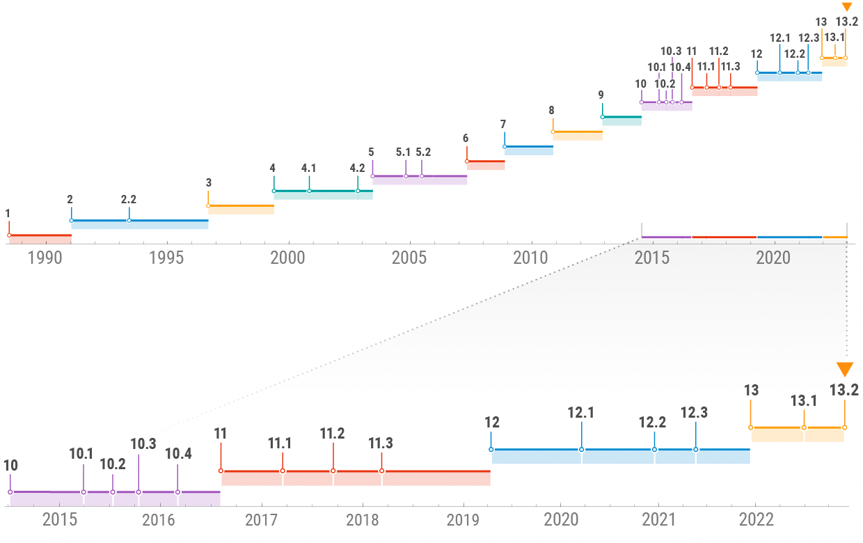
It’s been more than 35 years now since we released Version 1.0. And all those years we’ve been continuing to build a taller and taller tower of capabilities, progressively expanding the scope of our vision and the breadth of our computational coverage of the world:

Number of built-in fuctions

Version 1.0 had 554 built-in functions; in Version 14.0 there are 6602. And behind each of those functions is a story. Sometimes it’s a story of creating a superalgorithm that encapsulates decades of algorithmic development. Sometimes it’s a story of painstakingly curating data that’s never been assembled before. Sometimes it’s a story of drilling down to the essence of something to invent new approaches and new functions that can capture it.

And from all these pieces we’ve been steadily building the coherent whole that is today’s Wolfram Language. In the arc of intellectual history it defines a broad, new, computational paradigm for formalizing the world. And at a practical level it provides a superpower for implementing computational thinking—and enabling “computational X” for all fields X.

To us it’s profoundly satisfying to see what has been done over the past three decades with everything we’ve built so far. So many discoveries, so many inventions, so much achieved, so much learned. And seeing this helps drive forward our efforts to tackle still more, and to continue to push every boundary we can with our R&D, and to deliver the results in new versions of our system.

Our R&D portfolio is broad. From projects that get completed within months of their conception, to projects that rely on years (and sometimes even decades) of systematic development. And key to everything we do is leveraging what we have already done—often taking what in earlier years was a pinnacle of technical achievement, and now using it as a routine building block to reach a level that could barely even be imagined before. And beyond practical technology, we’re also continually going further and further in leveraging what’s now the vast conceptual framework that we’ve been building all these years—and progressively encapsulating it in the design of the Wolfram Language.

We’ve worked hard all these years not only to create ideas and technology, but also to craft a practical and sustainable ecosystem in which we can systematically do this now and into the long-term future. And we continue to innovate in these areas, broadening the delivery of what we’ve built in new and different ways, and through new and different channels. And in the past five years we’ve also been able to open up our core design process to the world—regularly livestreaming what we’re doing in a uniquely open way.

And indeed over the past several years the seeds of essentially everything we’re delivering today in Version 14.0 has been openly shared with the world, and represents an achievement not only for our internal teams but also for the many people who have participated in and commented on our livestreams.

Part of what Version 14.0 is about is continuing to expand the domain of our computational language, and our computational formalization of the world. But Version 14.0 is also about streamlining and polishing the functionality we’ve already defined. Throughout the system there are things we’ve made more efficient, more robust and more convenient. And, yes, in complex software, bugs of many kinds are a theoretical and practical inevitability. And in Version 14.0 we’ve fixed nearly 10,000 bugs, the majority found by our increasingly sophisticated internal software testing methods.

Now We Need to Tell the World

Even after all the work we’ve put into the Wolfram Language over the past several decades, there’s still yet another challenge: how to let people know just what the Wolfram Language can do. Back when we released Version 1.0 I was able to write a book of manageable size that could pretty much explain the whole system. But for Version 14.0—with all the functionality it contains—one would need a book with perhaps 200,000 pages.

And at this point nobody (even me!) immediately knows everything the Wolfram Language does. Of course one of our great achievements has been to maintain across all that functionality a tightly coherent and consistent design that results in there ultimately being only a small set of fundamental principles to learn. But at the vast scale of the Wolfram Language as it exists today, knowing what’s possible—and what can now be formulated in computational terms—is inevitably very challenging. And all too often when I show people what’s possible, I’ll get the response “I had no idea the Wolfram Language could do that!”

So in the past few years we’ve put increasing emphasis into building large-scale mechanisms to explain the Wolfram Language to people. It begins at a very fine-grained level, with “just-in-time information” provided, for example, through suggestions made when you type. Then for each function (or other construct in the language) there are pages that explain the function, with extensive examples. And now, increasingly, we’re adding “just-in-time learning material” that leverages the concreteness of the functions to provide self-contained explanations of the broader context of what they do.

By the way, in modern times we need to explain the Wolfram Language not just to humans, but also to AIs—and our very extensive documentation and examples have proved extremely valuable in training LLMs to use the Wolfram Language. And for AIs we’re providing a variety of tools—like immediate computable access to documentation, and computable error handling. And with our Chat Notebook technology there’s also a new “on ramp” for creating Wolfram Language code from linguistic (or visual, etc.) input.

But what about the bigger picture of the Wolfram Language? For both people and AIs it’s important to be able to explain things at a higher level, and we’ve been doing more and more in this direction. For more than 30 years we’ve had “guide pages” that summarize specific functionality in particular areas. Now we’re adding “core area pages” that give a broader picture of large areas of functionality—each one in effect covering what might otherwise be a whole product on its own, if it wasn’t just an integrated part of the Wolfram Language:

Core area pages

But we’re going even much further, building whole courses and books that provide modern hands-on Wolfram-Language-enabled introductions to a broad range of areas. We’ve now covered the material of many standard college courses (and quite a lot besides), in a new and very effective “computational” way, that allows immediate, practical engagement with concepts:

Wolfram U courses

All these courses involve not only lectures and notebooks but also auto-graded exercises, as well as official certifications. And we have a regular calendar of everyone-gets-together-at-the-same-time instructor-led peer Study Groups about these courses. And, yes, our Wolfram U operation is now emerging as a significant educational entity, with many thousands of students at any given time.

In addition to whole courses, we have “miniseries” of lectures about specific topics:

Miniseries video lectures

And we also have courses—and books—about the Wolfram Language itself, like my Elementary Introduction to the Wolfram Language, which came out in a third edition this year (and has an associated course, online version, etc.):

Elementary Introduction to the Wolfram Language

In a somewhat different direction, we’ve expanded our Wolfram Summer School to add a Wolfram Winter School, and we’ve greatly expanded our Wolfram High School Summer Research Program, adding year-round programs, middle-school programs, etc.—including the new “Computational Adventures” weekly activity program.

And then there’s livestreaming. We’ve been doing weekly “R&D livestreams” with our development team (and sometimes also external guests). And I myself have also been doing a lot of livestreaming (232 hours of it in 2023 alone)—some of it design reviews of Wolfram Language functionality, and some of it answering questions, technical and other.

The list of ways we’re getting the word out about the Wolfram Language goes on. There’s Wolfram Community, that’s full of interesting contributions, and has ever-increasing readership. There are sites like Wolfram Challenges. There are our Wolfram Technology Conferences. And lots more.

We’ve put immense effort into building the whole Wolfram technology stack over the past four decades. And even as we continue to aggressively build it, we’re putting more and more effort into telling the world about just what’s in it, and helping people (and AIs) to make the most effective use of it. But in a sense, everything we’re doing is just a seed for what the wider community of Wolfram Language users are doing, and can do. Spreading the power of the Wolfram Language to more and more people and areas.

The LLMs Have Landed

The machine learning superfunctions Classify and Predict first appeared in Wolfram Language in 2014 (Version 10). By the next year there were starting to be functions like ImageIdentify and LanguageIdentify, and within a couple of years we’d introduced our whole neural net framework and Neural Net Repository. Included in that were a variety of neural nets for language modeling, that allowed us to build out functions like SpeechRecognize and an experimental version of FindTextualAnswer. But—like everyone else—we were taken by surprise at the end of 2022 by ChatGPT and its remarkable capabilities.

Very quickly we realized that a major new use case—and market—had arrived for Wolfram|Alpha and Wolfram Language. For now it was not only humans who’d need the tools we’d built; it was also AIs. By March 2023 we’d worked with OpenAI to use our Wolfram Cloud technology to deliver a plugin to ChatGPT that allows it to call Wolfram|Alpha and Wolfram Language. LLMs like ChatGPT provide remarkable new capabilities in reproducing human language, basic human thinking and general commonsense knowledge. But—like unaided humans—they’re not set up to deal with detailed computation or precise knowledge. For that, like humans, they have to use formalism and tools. And the remarkable thing is that the formalism and tools we’ve built in Wolfram Language (and Wolfram|Alpha) are basically a broad, perfect fit for what they need.

We created the Wolfram Language to provide a bridge from what humans think about to what computation can express and implement. And now that’s what the AIs can use as well. The Wolfram Language provides a medium not only for humans to “think computationally” but also for AIs to do so. And we’ve been steadily doing the engineering to let AIs call on Wolfram Language as easily as possible.

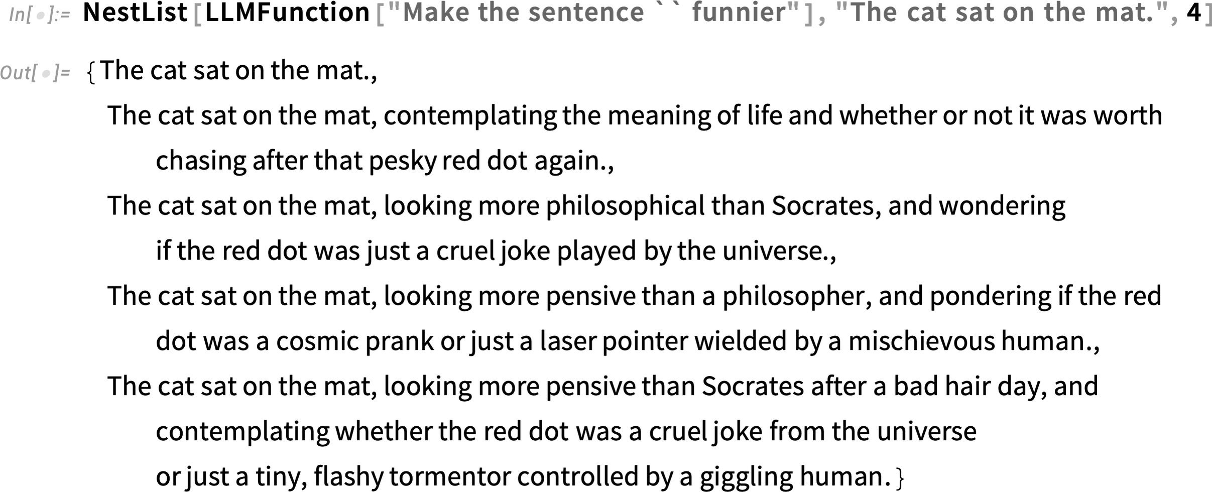
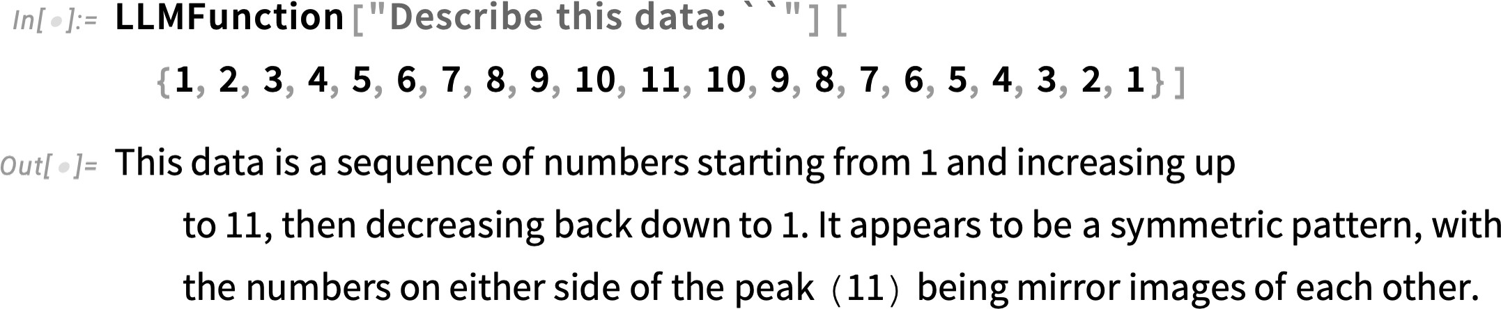
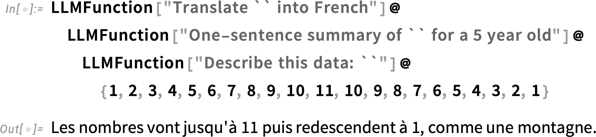
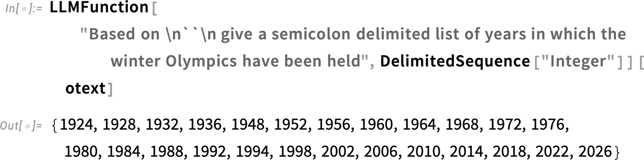
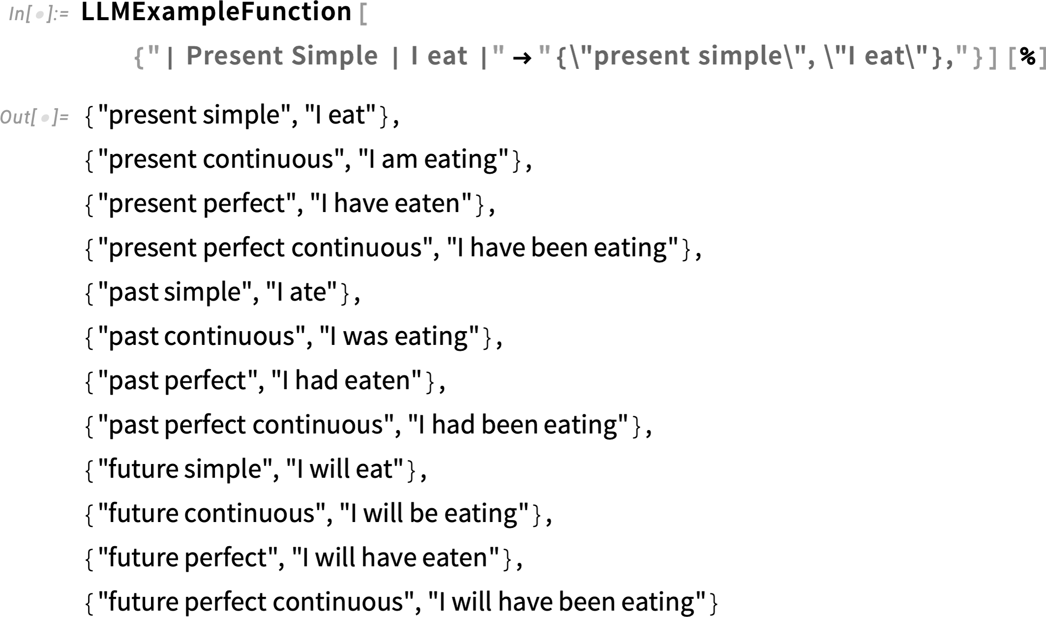
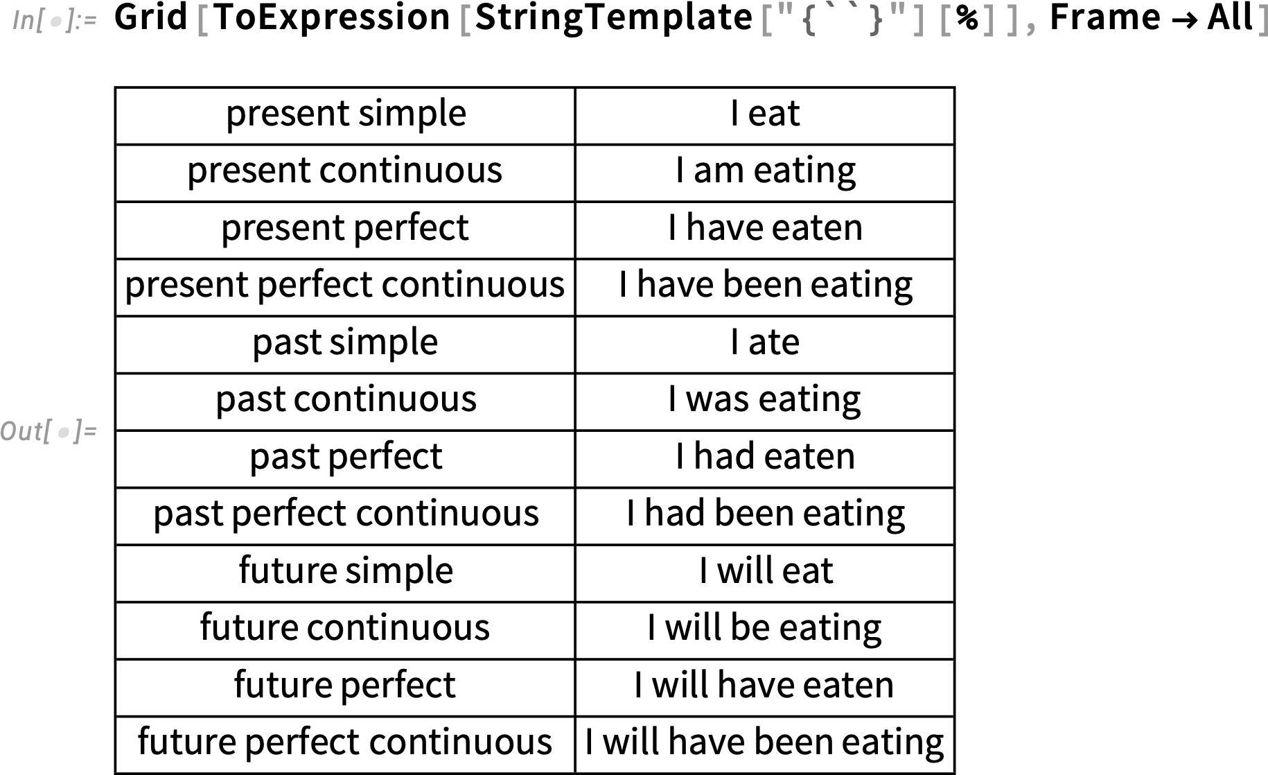
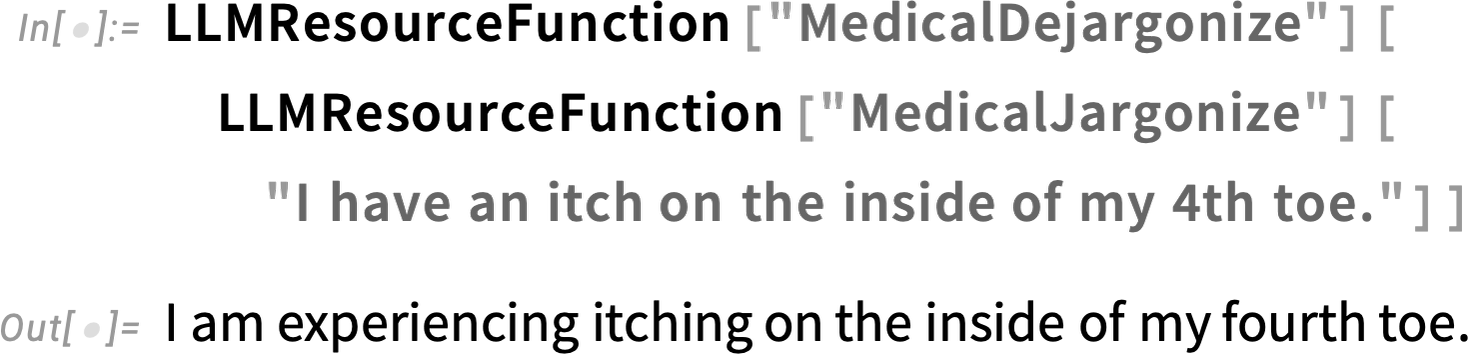
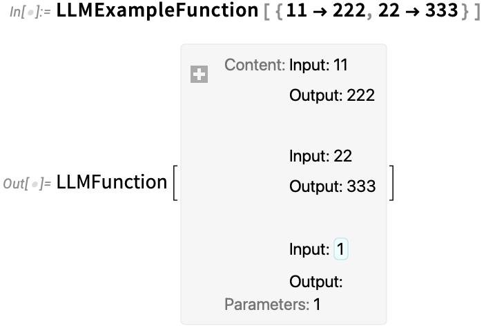
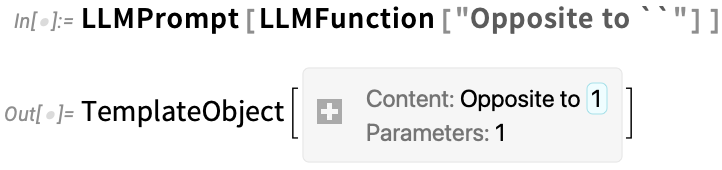
But in addition to LLMs using Wolfram Language, there’s also now the possibility of Wolfram Language using LLMs. And already in June 2023 (Version 13.3) we released a major collection of LLM-based capabilities in Wolfram Language. One category is LLM functions, that effectively use LLMs as “internal algorithms” for operations in Wolfram Language:

In typical Wolfram Language fashion, we have a symbolic representation for LLMs: LLMConfiguration[] represents an LLM with its various parameters, promptings, etc. And in the past few months we’ve been steadily adding connections to the full range of popular LLMs, making Wolfram Language a unique hub not only for LLM usage, but also for studying the performance—and science—of LLMs.

You can define your own LLM functions in Wolfram Language. But there’s also the Wolfram Prompt Repository that plays a similar role for LLM functions as the Wolfram Function Repository does for ordinary Wolfram Language functions. There’s a public Prompt Repository that so far has several hundred curated prompts. But it’s also possible for anyone to post their prompts in the Wolfram Cloud and make them publicly (or privately) accessible. The prompts can define personas (“talk like a [stereotypical] pirate”). They can define AI-oriented functions (“write it with emoji”). And they can define modifiers that affect the form of output (“haiku style”).

Wolfram Prompt Repository

In addition to calling LLMs “programmatically” within Wolfram Language, there’s the new concept (first introduced in Version 13.3) of “Chat Notebooks”. Chat Notebooks represent a new kind of user interface, that combines the graphical, computational and document features of traditional Wolfram Notebooks with the new linguistic interface capabilities brought to us by LLMs.

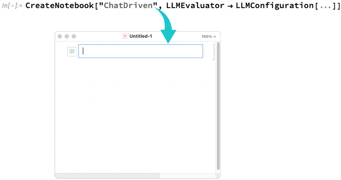
The basic idea of a Chat Notebook—as introduced in Version 13.3, and now extended in Version 14.0—is that you can have “chat cells” (requested by typing ) whose content gets sent not to the Wolfram kernel, but instead to an LLM:

Write a haiku about a crocodile on the moon

You can use “function prompts”—say from the Wolfram Prompt Repository—directly in a Chat Notebook:

A cat ate my lunch

And as of Version 14.0 you can also knit Wolfram Language computations directly into your “conversation” with the LLM:

Make a haiku from RandomWord

(You type \ to insert Wolfram Language, very much like the way you can use <**> to insert Wolfram Language into external evaluation cells.)

One thing about Chat Notebooks is that—as their name suggests—they really are centered around “chatting”, and around having a sequential interaction with an LLM. In an ordinary notebook, it doesn’t matter where in the notebook each Wolfram Language evaluation is requested; all that’s relevant is the order in which the Wolfram kernel does the evaluations. But in a Chat Notebook the “LLM evaluations” are always part of a “chat” that’s explicitly laid out in the notebook.

A key part of Chat Notebooks is the concept of a chat block: type ~ and you get a separator in the notebook that “starts a new chat”:

My name is Stephen

Chat Notebooks—with all their typical Wolfram Notebook editing, structuring, automation, etc. capabilities—are very powerful just as “LLM interfaces”. But there’s another dimension as well, enabled by LLMs being able to call Wolfram Language as a tool.

At one level, Chat Notebooks provide an “on ramp” for using Wolfram Language. Wolfram|Alpha—and even more so, Wolfram|Alpha Notebook Edition—let you ask questions in natural language, then have the questions translated into Wolfram Language, and answers computed. But in Chat Notebooks you can go beyond asking specific questions. Instead, through the LLM, you can just “start chatting” about what you want to do, then have Wolfram Language code generated, and executed:

How do you make a rosette with 5 lobes?

The workflow is typically as follows. First, you have to conceptualize in computational terms what you want. (And, yes, that step requires computational thinking—which is a very important skill that too few people have so far learned.) Then you tell the LLM what you want, and it’ll try to write Wolfram Language code to achieve it. It’ll typically run the code for you (but you can also always do it yourself)—and you can see whether you got what you wanted. But what’s crucial is that Wolfram Language is intended to be read not only by computers but also by humans. And particularly since LLMs actually usually seem to manage to write pretty good Wolfram Language code, you can expect to read what they wrote, and see if it’s what you wanted. If it is, you can take that code, and use it as a “solid building block” for whatever larger system you might be trying to set up. Otherwise, you can either fix it yourself, or try chatting with the LLM to get it to do it.

One of the things we see in the example above is the LLM—within the Chat Notebook—making a “tool call”, here to a Wolfram Language evaluator. In the Wolfram Language there’s now a whole mechanism for defining tools for LLMs—with each tool being represented by an LLMTool symbolic object. In Version 14.0 there’s an experimental version of the new Wolfram LLM Tool Repository with some predefined tools:

Wolfram LLM Tool Repository

In a default Chat Notebook, the LLM has access to some default tools, which include not only the Wolfram Language evaluator, but also things like Wolfram documentation search and Wolfram|Alpha query. And it’s common to see the LLM go back and forth trying to write “code that works”, and for example sometimes having to “resort” (much like humans do) to reading the documentation.

Something that’s new in Version 14.0 is experimental access to multimodal LLMs that can take images as well as text as input. And when this capability is enabled, it allows the LLM to “look at pictures from the code it generated”, see if they’re what was asked for, and potentially correct itself:

Create graphics with a randomly colored disc

The deep integration of images into Wolfram Language—and Wolfram Notebooks—yields all sorts of possibilities for multimodal LLMs. Here we’re giving a plot as an image and asking the LLM how to reproduce it:

Create a similar plot

Another direction for multimodal LLMs is to take data (in the hundreds of formats accepted by Wolfram Language) and use the LLM to guide its visualization and analysis in the Wolfram Language. Here’s an example that starts from a file data.csv in the current directory on your computer:

Look at the file data.csv

One thing that’s very nice about using Wolfram Language directly is that everything you do (well, unless you use RandomInteger, etc.) is completely reproducible; do the same computation twice and you’ll get the same result. That’s not true with LLMs (at least right now). And so when one uses LLMs it feels like something more ephemeral and fleeting than using Wolfram Language. One has to grab any good results one gets—because one might never be able to reproduce them. Yes, it’s very helpful that one can store everything in a Chat Notebook, even if one can’t rerun it and get the same results. But the more “permanent” use of LLM results tends to be “offline”. Use an LLM “up front” to figure something out, then just use the result it gave.

One unexpected application of LLMs for us has been in suggesting names of functions. With the LLM’s “experience” of what people talk about, it’s in a good position to suggest functions that people might find useful. And, yes, when it writes code it has a habit of hallucinating such functions. But in Version 14.0 we’ve actually added one function—DigitSum—that was suggested to us by LLMs. And in a similar vein, we can expect LLMs to be useful in making connections to external databases, functions, etc. The LLM “reads the documentation”, and tries to write Wolfram Language “glue” code—which then can be reviewed, checked, etc., and if it’s right, can be used henceforth.

Then there’s data curation, which is a field that—through Wolfram|Alpha and many of our other efforts—we’ve become extremely expert at over the past couple of decades. How much can LLMs help with that? They certainly don’t “solve the whole problem”, but integrating them with the tools we already have has allowed us over the past year to speed up some of our data curation pipelines by factors of two or more.

If we look at the whole stack of technology and content that’s in the modern Wolfram Language, the overwhelming majority of it isn’t helped by LLMs, and isn’t likely to be. But there are many—sometimes unexpected—corners where LLMs can dramatically improve heuristics or otherwise solve problems. And in Version 14.0 there are starting to be a wide variety of “LLM inside” functions.

An example is TextSummarize, which is a function we’ve considered adding for many versions—but now, thanks to LLMs, can finally implement to a useful level:

The main LLMs that we’re using right now are based on external services. But we’re building capabilities to allow us to run LLMs in local Wolfram Language installations as soon as that’s technically feasible. And one capability that’s actually part of our mainline machine learning effort is NetExternalObject—a way of representing symbolically an externally defined neural net that can be run inside Wolfram Language. NetExternalObject allows you, for example, to take any network in ONNX form and effectively treat it as a component in a Wolfram Language neural net. Here’s a network for image depth estimation—that we’re here importing from an external repository (though in this case there’s actually a similar network already in the Wolfram Neural Net Repository):

Now we can apply this imported network to an image that’s been encoded with our built-in image encoder—then we’re taking the result and visualizing it:

It’s often very convenient to be able to run networks locally, but it can sometimes take quite high-end hardware to do so. For example, there’s now a function in the Wolfram Function Repository that does image synthesis entirely locally—but to run it, you do need a GPU with at least 8 GB of VRAM:

By the way, based on LLM principles (and ideas like transformers) there’ve been other related advances in machine learning that have been strengthening a whole range of Wolfram Language areas—with one example being image segmentation, where ImageSegmentationComponents now provides robust “content-sensitive” segmentation:

Still Going Strong on Calculus

When Mathematica 1.0 was released in 1988, it was a “wow” that, yes, now one could routinely do integrals symbolically by computer. And it wasn’t long before we got to the point—first with indefinite integrals, and later with definite integrals—where what’s now the Wolfram Language could do integrals better than any human. So did that mean we were “finished” with calculus? Well, no. First there were differential equations, and partial differential equations. And it took a decade to get symbolic ODEs to a beyond-human level. And with symbolic PDEs it took until just a few years ago. Somewhere along the way we built out discrete calculus, asymptotic expansions and integral transforms. And we also implemented lots of specific features needed for applications like statistics, probability, signal processing and control theory. But even now there are still frontiers.

And in Version 14 there are significant advances around calculus. One category concerns the structure of answers. Yes, one can have a formula that correctly represents the solution to a differential equation. But is it in the best, simplest or most useful form? Well, in Version 14 we’ve worked hard to make sure it is—often dramatically reducing the size of expressions that get generated.

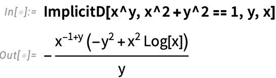
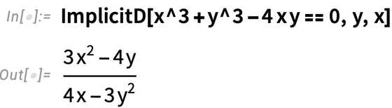
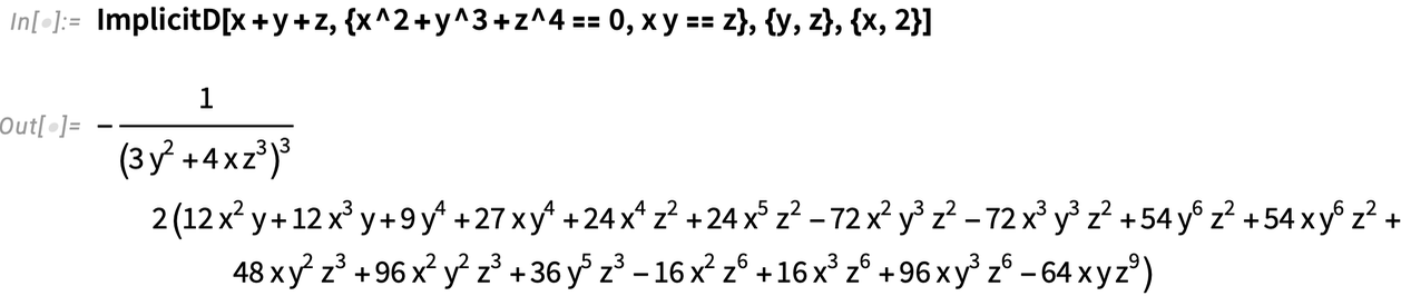
Another advance has to do with expanding the range of “pre-packaged” calculus operations. We’ve been able to do derivatives ever since Version 1.0. But in Version 14 we’ve added implicit differentiation. And, yes, one can give a basic definition for this easily enough using ordinary differentiation and equation solving. But by adding an explicit ImplicitD we’re packaging all that up—and handling the tricky corner cases—so that it becomes routine to use implicit differentiation wherever you want:

Another category of pre-packaged calculus operations new in Version 14 are ones for vector-based integration. These were always possible to do in a “do-it-yourself” mode. But in Version 14 they are now streamlined built-in functions—that, by the way, also cover corner cases, etc. And what made them possible is actually a development in another area: our decade-long project to add geometric computation to Wolfram Language—which gave us a natural way to describe geometric constructs such as curves and surfaces:


Related functionality new in Version 14 is ContourIntegrate:

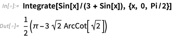
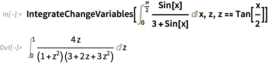
Functions like ContourIntegrate just “get the answer”. But if one’s learning or exploring calculus it’s often also useful to be able to do things in a more step-by-step way. In Version 14 you can start with an inactive integral

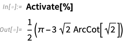
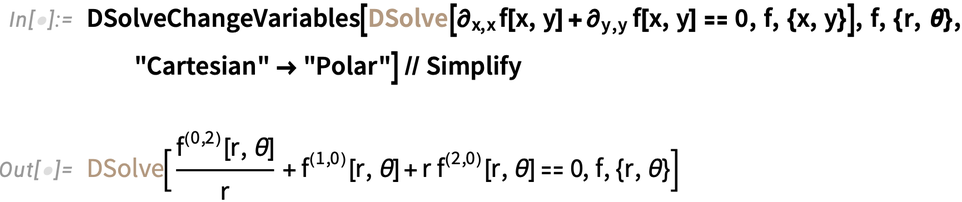
and explicitly do operations like changing variables:

Sometimes actual answers get expressed in inactive form, particularly as infinite sums:

And now in Version 14 the function TruncateSum lets you take such a sum and generate a truncated “approximation”:

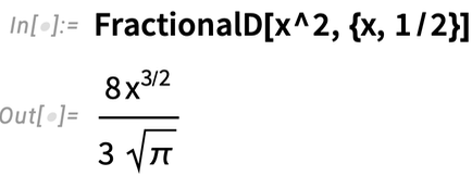
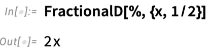
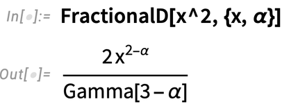
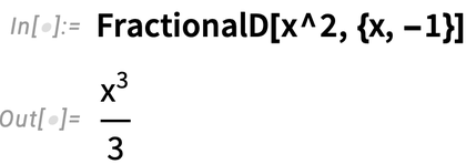
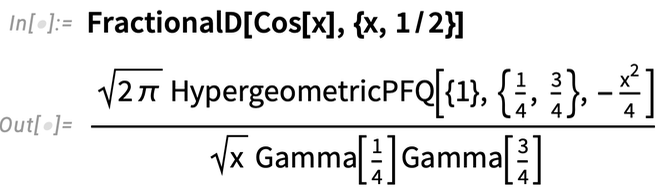
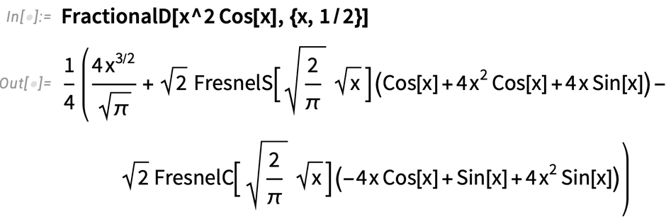
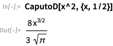
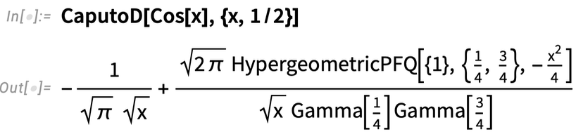
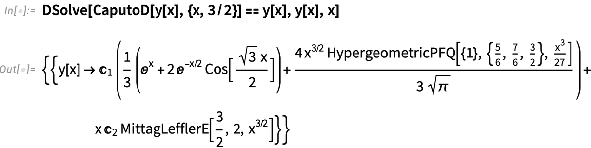
Functions like D and Integrate—as well as LineIntegrate and SurfaceIntegrate—are, in a sense, “classic calculus”, taught and used for more than three centuries. But in Version 14 we also support what we can think of as “emerging” calculus operations, like fractional differentiation:

Core Language

What are the primitives from which we can best build our conception of computation? That’s at some level the question I’ve been asking for more than four decades, and what’s determined the functions and structures at the core of the Wolfram Language.

And as the years go by, and we see more and more of what’s possible, we recognize and invent new primitives that will be useful. And, yes, the world—and the ways people interact with computers—change too, opening up new possibilities and bringing new understanding of things. Oh, and this year there are LLMs which can “get the intellectual sense of the world” and suggest new functions that can fit into the framework we’ve created with the Wolfram Language. (And, by the way, there’ve also been lots of great suggestions made by the audiences of our design review livestreams.)

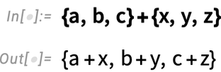
One new construct added in Version 13.1—and that I personally have found very useful—is Threaded. When a function is listable—as Plus is—the top levels of lists get combined:

But sometimes you want one list to be “threaded into” the other at the lowest level, not the highest. And now there’s a way to specify that, using Threaded:

In a sense, Threaded is part of a new wave of symbolic constructs that have “ambient effects” on lists. One very simple example (introduced in 2015) is Nothing:

Another, introduced in 2020, is Splice:

An old chestnut of Wolfram Language design concerns the way infinite evaluation loops are handled. And in Version 13.2 we introduced the symbolic construct TerminatedEvaluation to provide better definition of how out-of-control evaluations have been terminated:
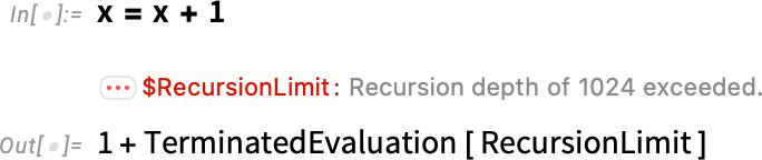
In a curious connection, in the computational representation of physics in our recent Physics Project, the direct analog of nonterminating evaluations are what make possible the seemingly unending universe in which we live.

But what is actually going on “inside an evaluation”, terminating or not? I’ve always wanted a good representation of this. And in fact back in Version 2.0 we introduced Trace for this purpose:

But just how much detail of what the evaluator does should one show? Back in Version 2.0 we introduced the option TraceOriginal that traces every path followed by the evaluator:

But often this is way too much. And in Version 14.0 we’ve introduced the new setting TraceOriginalAutomatic, which doesn’t include in its output evaluations that don’t do anything:

This may seem pedantic, but when one has an expression of any substantial size, it’s a crucial piece of pruning. So, for example, here’s a graphical representation of a simple arithmetic evaluation, with TraceOriginalTrue:

And here’s the corresponding “pruned” version, with TraceOriginalAutomatic:

(And, yes, the structures of these graphs are closely related to things like the causal graphs we construct in our Physics Project.)

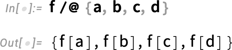
In the effort to add computational primitives to the Wolfram Language, two new entrants in Version 14.0 are Comap and ComapApply. The function Map takes a function f and “maps it” over a list:

Comap does the “mathematically co-” version of this, taking a list of functions and “comapping” them onto a single argument:

Why is this useful? As an example, one might want to apply three different statistical functions to a single list. And now it’s easy to do that, using Comap:

By the way, as with Map, there’s also an operator form for Comap:

Comap works well when the functions it’s dealing with take just one argument. If one has functions that take multiple arguments, ComapApply is what one typically wants:

Talking of “co-like” functions, a new function added in Version 13.2 is PositionSmallest. Min gives the smallest element in a list; PositionSmallest instead says where the smallest elements are:

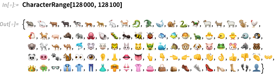
One of the important objectives in the Wolfram Language is to have as much as possible “just work”. When we released Version 1.0 strings could be assumed just to contain ordinary ASCII characters, or perhaps to have an external character encoding defined. And, yes, it could be messy not to know “within the string itself” what characters were supposed to be there. And by the time of Version 3.0 in 1996 we’d become contributors to, and early adopters of, Unicode, which provided a standard encoding for “16-bits’-worth” of characters. And for many years this served us well. But in time—and particularly with the growth of emoji—16 bits wasn’t enough to encode all the characters people wanted to use. So a few years ago we began rolling out support for 32-bit Unicode, and in Version 13.1 we integrated it into notebooks—in effect making strings something much richer than before:

And, yes, you can use Unicode everywhere now:

Video as a Fundamental Object

Back when Version 1.0 was released, a megabyte was a lot of memory. But 35 years later we routinely deal with gigabytes. And one of the things that makes practical is computation with video. We first introduced Video experimentally in Version 12.1 in 2020. And over the past three years we’ve been systematically broadening and strengthening our ability to deal with video in Wolfram Language. Probably the single most important advance is that things around video now—as much as possible—“just work”, without “creaking” under the strain of handling such large amounts of data.

We can directly capture video into notebooks, and we can robustly play video anywhere within a notebook. We’ve also added options for where to store the video so that it’s conveniently accessible to you and anyone else you want to give access to it.

There’s lots of complexity in the encoding of video—and we now robustly and transparently support more than 500 codecs. We also do lots of convenient things automatically, like rotating portrait-mode videos—and being able to apply image processing operations like ImageCrop across whole videos. In every version, we’ve been further optimizing the speed of some video operation or another.

But a particularly big focus has been on video generators: programmatic ways to produce videos and animations. One basic example is AnimationVideo, which produces the same kind of output as Animate, but as a Video object that can either be displayed directly in a notebook, or exported in MP4 or some other format:

AnimationVideo

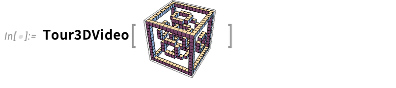
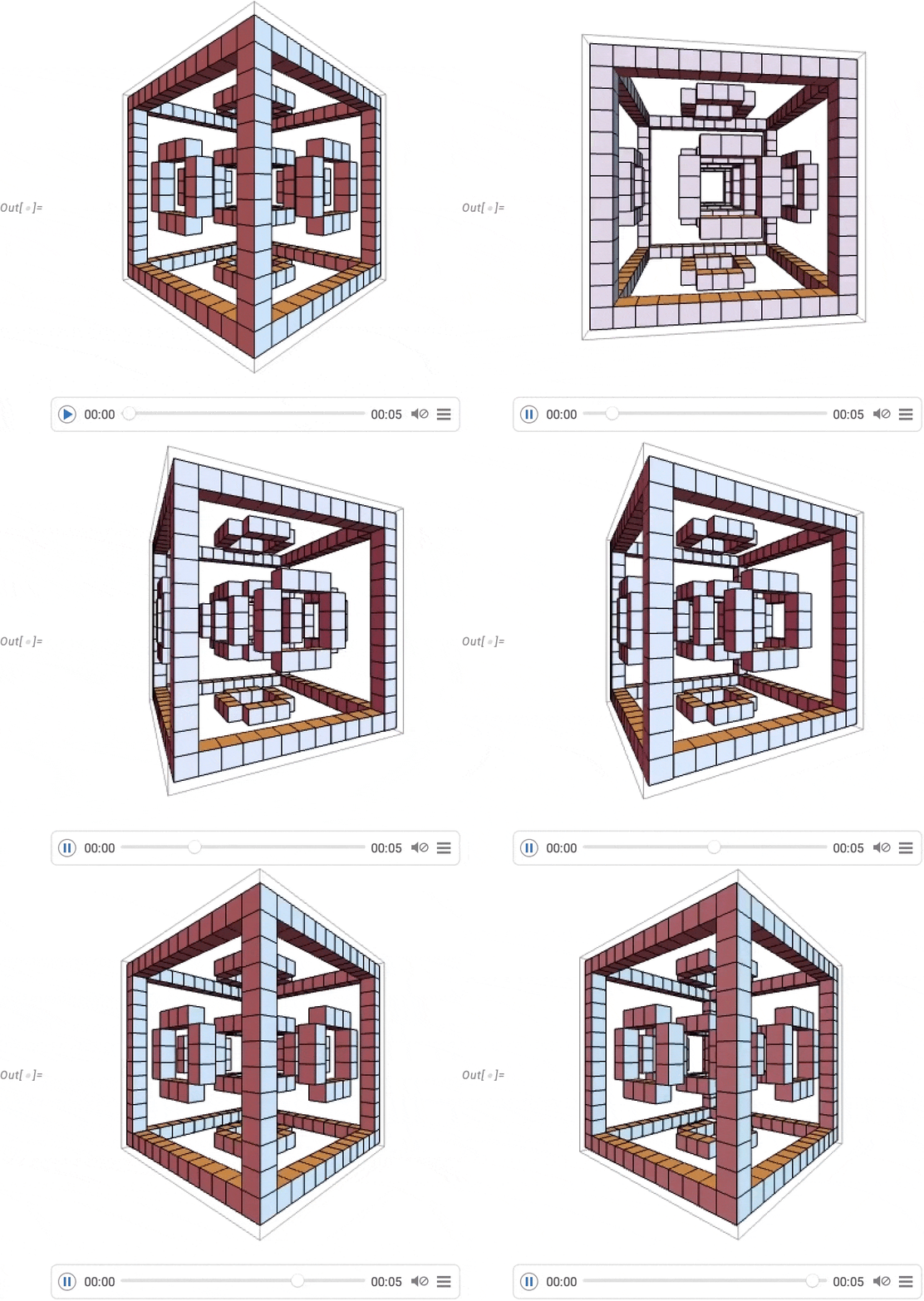
AnimationVideo is based on computing each frame in a video by evaluating an expression. Another class of video generators take an existing visual construct, and simply “tour” it. TourVideo “tours” images, graphics and geo graphics; Tour3DVideo (new in Version 14.0) tours 3D geometry:
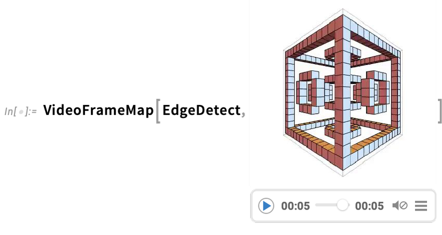
A very powerful capability in Wolfram Language is being able to apply arbitrary functions to videos. One example of how this can be done is VideoFrameMap, which maps a function across frames of a video, and which was made efficient in Version 13.2:
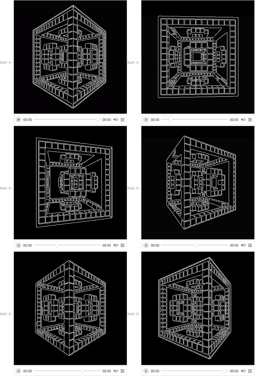
And although Wolfram Language isn’t intended as an interactive video editing system, we’ve made sure that it’s possible to do streamlined programmatic video editing in the language, and for example in Version 14.0 we’ve added things like transition effects in VideoJoin and timed overlays in OverlayVideo.

So Much Got Faster, Stronger, Sleeker

With every new version of Wolfram Language we add new capabilities to extend yet further the domain of the language. But we also put a lot of effort into something less immediately visible: making existing capabilities faster, stronger and sleeker.

And in Version 14 two areas where we can see some examples of all these are dates and quantities. We introduced the notion of symbolic dates (DateObject, etc.) nearly a decade ago. And over the years since then we’ve built many things on this structure. And in the process of doing this it’s become clear that there are certain flows and paths that are particularly common and convenient. At the beginning what mattered most was just to make sure that the relevant functionality existed. But over time we’ve been able to see what should be streamlined and optimized, and we’ve steadily been doing that.

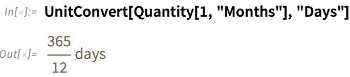
In addition, as we’ve worked towards new and different applications, we’ve seen “corners” that need to be filled in. So, for example, astronomy is an area we’ve significantly developed in Version 14, and supporting astronomy has required adding several new “high-precision” time capabilities, such as the TimeSystem option, as well as new astronomy-oriented calendar systems. Another example concerns date arithmetic. What should happen if you want to add a month to January 30? Where should you land? Different kinds of business applications and contracts make different assumptions—and so we added a Method option to functions like DatePlus to handle this. Meanwhile, having realized that date arithmetic is involved in the “inner loop” of certain computations, we optimized it—achieving a more than 100x speedup in Version 14.0.

Wolfram|Alpha has been able to deal with units ever since it was first launched in 2009—now more than 10,000 of them. And in 2012 we introduced Quantity to represent quantities with units in the Wolfram Language. And over the past decade we’ve been steadily smoothing out a whole series of complicated gotchas and issues with units. For example, what does 100°C + 20°C mean? Well, the 20°C isn’t really the same kind of thing as the 100°C. And now in Wolfram Language we have a systematic way to handle this, by distinguishing temperature and temperature difference units—so that we now write 100°C + .

At first our priority with Quantity was to get it working as broadly as possible, and to integrate it as widely as possible into computations, visualizations, etc. across the system. But as its capabilities have expanded, so have its uses, repeatedly driving the need to optimize its operation for particular common cases. And indeed between Version 13 and Version 14 we’ve dramatically sped up many things related to Quantity, often by factors of 1000 or more.

Talking of speedups, another example—made possible by new algorithms operating on multithreaded CPUs—concerns polynomials. We’ve worked with polynomials in Wolfram Language since Version 1, but in Version 13.2 there was a dramatic speedup of up to 1000x on operations like polynomial factoring.

In addition, a new algorithm in Version 14.0 dramatically speeds up numerical solutions to polynomial and transcendental equations—and, together with the new MaxRoots options, allows us, for example, to pick off a few roots from a degree-one-million polynomial

or to find roots of a transcendental equation that we could not even attempt before without pre-specifying bounds on their values:

Another “old” piece of functionality with recent enhancement concerns mathematical functions. Ever since Version 1.0 we’ve set up mathematical functions so that they can be computed to arbitrary precision:

But in recent versions we’ve wanted to be “more precise about precision”, and to be able to rigorously compute just what range of outputs are possible given the range of values provided as input:

But every function for which we do this effectively requires a new theorem, and we’ve been steadily increasing the number of functions covered—now more than 130—so that this “just works” when you need to use it in a computation.

The Tree Story Continues

Trees are useful. We first introduced them as basic objects in the Wolfram Language only in Version 12.3. But now that they’re there, we’re discovering more and more places they can be used. And to support that, we’ve been adding more and more capabilities to them.

One area that’s advanced significantly since Version 13 is the rendering of trees. We tightened up the general graphic design, but, more importantly, we introduced many new options for how rendering should be done.

For example, here’s a random tree where we’ve specified that for all nodes only 3 children should be explicitly displayed: the others are elided away:

Here we’re adding several options to define the rendering of the tree:

By default, the branches in trees are labeled with integers, just like parts in an expression. But in Version 13.1 we added support for named branches defined by associations:

Our original conception of trees was very centered around having elements one would explicitly address, and that could have “payloads” attached. But what became clear is that there were applications where all that mattered was the structure of the tree, not anything about its elements. So we added UnlabeledTree to create “pure trees”:

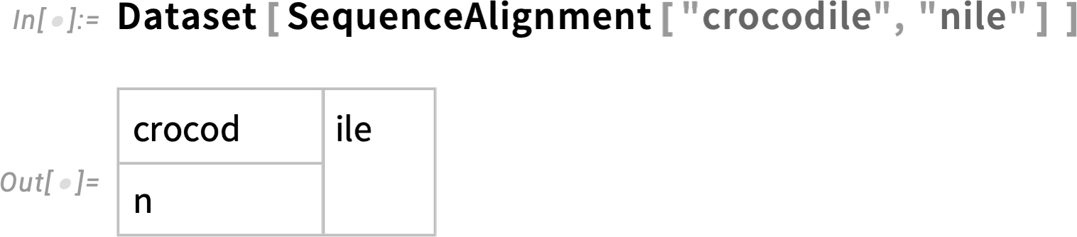
Trees are useful because many kinds of structures are basically trees. And since Version 13 we’ve added capabilities for converting trees to and from various kinds of structures. For example, here’s a simple Dataset object:

You can use ExpressionTree to convert this to a tree:

And TreeExpression to convert it back:

We’ve also added capabilities for converting to and from JSON and XML, as well as for representing file directory structures as trees:

Finite Fields

In Version 1.0 we had integers, rational numbers and real numbers. In Version 3.0 we added algebraic numbers (represented implicitly by Root)—and a dozen years later we added algebraic number fields and transcendental roots. For Version 14 we’ve now added another (long-awaited) “number-related” construct: finite fields.

Here’s our symbolic representation of the field of integers modulo 7:

And now here’s a specific element of that field

which we can immediately compute with:

But what’s really important about what we’ve done with finite fields is that we’ve fully integrated them into other functions in the system. So, for example, we can factor a polynomial whose coefficients are in a finite field:

We can also do things like find solutions to equations over finite fields. So here, for example, is a point on a Fermat curve over the finite field GF(173):

And here is a power of a matrix with elements over the same finite field:

Going Off Planet: The Astro Story

A major new capability added since Version 13 is astro computation. It begins with being able to compute to high precision the positions of things like planets. Even knowing what one means by “position” is complicated, though—with lots of different coordinate systems to deal with. By default AstroPosition gives the position in the sky at the current time from your Here location:

But one can instead ask about a different coordinate system, like global galactic coordinates:

And now here’s a plot of the distance between Saturn and Jupiter over a 50-year period:

In direct analogy to GeoGraphics, we’ve added AstroGraphics, here showing a patch of sky around the current position of Saturn:

And this now shows the sequence of positions for Saturn over the course of a couple of years—yes, including retrograde motion:

There are many styling options for AstroGraphics. Here we’re adding a background of the “galactic sky”:

And here we’re including renderings for constellations (and, yes, we had an artist draw them):

Something specifically new in Version 14.0 has to do with extended handling of solar eclipses. We always try to deliver new functionality as fast as we can. But in this case there was a very specific deadline: the total solar eclipse visible from the US on April 8, 2024. We’ve had the ability to do global computations about solar eclipses for some time (actually since soon before the 2017 eclipse). But now we can also do detailed local computations right in the Wolfram Language.

So, for example, here’s a somewhat detailed overall map of the April 8, 2024, eclipse:

Now here’s a plot of the magnitude of the eclipse over a few hours, complete with a little “rampart” associated with the period of totality:

And here’s a map of the region of totality every minute just after the moment of maximum eclipse:

Millions of Species Become Computable

We first introduced computable data on biological organisms back when Wolfram|Alpha was released in 2009. But in Version 14—following several years of work—we’ve dramatically broadened and deepened the computable data we have about biological organisms.

So for example here’s how we can figure out what species have cheetahs as predators:

And here are pictures of these:

Here’s a map of countries where cheetahs have been seen (in the wild):

We now have data—curated from a great many sources—on more than a million species of animals, as well as most of the plants, fungi, bacteria, viruses and archaea that have been described. And for animals, for example, we have nearly 200 properties that are extensively filled in. Some are taxonomic properties:

Some are physical properties:

Some are genetic properties:

Some are ecological properties (yes, the cheetah is not the apex predator):

It’s useful to be able to get properties of individual species, but the real power of our curated computable data shows up when one does larger-scale analyses. Like here’s a plot of the lengths of genomes for organisms with the longest ones across our collection of organisms:

Or here’s a histogram of the genome lengths for organisms in the human gut microbiome:

And here’s a scatterplot of the lifespans of birds against their weights:

Following the idea that cheetahs aren’t apex predators, this is a graph of what’s “above” them in the food chain:

Chemical Computation

We began the process of introducing chemical computation into the Wolfram Language in Version 12.0, and by Version 13 we had good coverage of atoms, molecules, bonds and functional groups. Now in Version 14 we’ve added coverage of chemical formulas, amounts of chemicals—and chemical reactions.

Here’s a chemical formula, that basically just gives a “count of atoms”:

Now here are specific molecules with that formula:

Let’s pick one of these molecules:

Now in Version 14 we have a way to represent a certain quantity of molecules of a given type—here 1 gram of methylcyclopentane:

ChemicalConvert can convert to a different specification of quantity, here moles:

And here a count of molecules:

But now the bigger story is that in Version 14 we can represent not just individual types of molecules, and quantities of molecules, but also chemical reactions. Here we give a “sloppy” unbalanced representation of a reaction, and ReactionBalance gives us the balanced version:

And now we can extract the formulas for the reactants:

We can also give a chemical reaction in terms of molecules:

But with our symbolic representation of molecules and reactions, there’s now a big thing we can do: represent classes of reactions as “pattern reactions”, and work with them using the same kinds of concepts as we use in working with patterns for general expressions. So, for example, here’s a symbolic representation of the hydrohalogenation reaction:

Now we can apply this pattern reaction to particular molecules:

Here’s a more elaborate example, in this case entered using a SMARTS string:

Here we’re applying the reaction just once:

And now we’re doing it repeatedly
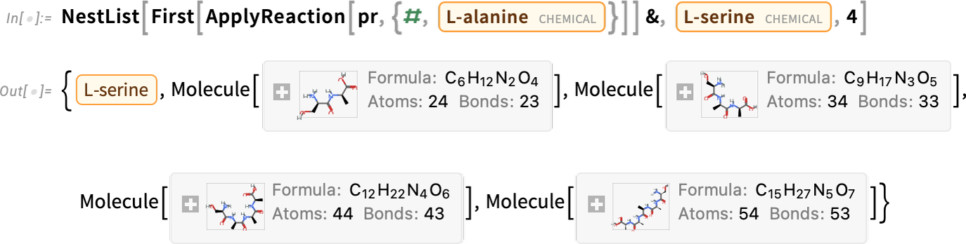
in this case generating longer and longer molecules (which in this case happen to be polypeptides):

The Knowledgebase Is Always Growing

Every minute of every day, new data is being added to the Wolfram Knowledgebase. Much of it is coming automatically from real-time feeds. But we also have a very large-scale ongoing curation effort with humans in the loop. We’ve built sophisticated (Wolfram Language) automation for our data curation pipeline over the years—and this year we’ve been able to increase efficiency in some areas by using LLM technology. But it’s hard to do curation right, and our long-term experience is that to do so ultimately requires human experts being in the loop, which we have.

So what’s new since Version 13.0? 291,842 new notable current and historical people; 264,467 music works; 118,538 music albums; 104,024 named stars; and so on. Sometimes the addition of an entity is driven by the new availability of reliable data; often it’s driven by the need to use that entity in some other piece of functionality (e.g. stars to render in AstroGraphics). But more than just adding entities there’s the issue of filling in values of properties of existing entities. And here again we’re always making progress, sometimes integrating newly available large-scale secondary data sources, and sometimes doing direct curation ourselves from primary sources.

A recent example where we needed to do direct curation was in data on alcoholic beverages. We have very extensive data on hundreds of thousands of types of foods and drinks. But none of our large-scale sources included data on alcoholic beverages. So that’s an area where we need to go to primary sources (in this case typically the original producers of products) and curate everything for ourselves.

So, for example, we can now ask for something like the distribution of flavors of different varieties of vodka (actually, personally, not being a consumer of such things, I had no idea vodka even had flavors…):

But beyond filling out entities and properties of existing types, we’ve also steadily been adding new entity types. One recent example is geological formations, 13,706 of them:

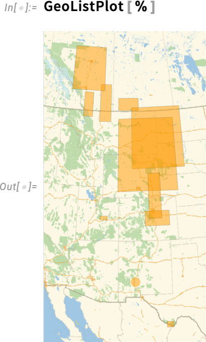
So now, for example, we can specify where T. rex have been found

and we can show those regions on a map:
Industrial-Strength Multidomain PDEs

PDEs are hard. It’s hard to solve them. And it’s hard to even specify what exactly you want to solve. But we’ve been on a multi-decade mission to “consumerize” PDEs and make them easier to work with. Many things go into this. You need to be able to easily specify elaborate geometries. You need to be able to easily define mathematically complicated boundary conditions. You need to have a streamlined way to set up the complicated equations that come out of underlying physics. Then you have to—as automatically as possible—do the sophisticated numerical analysis to efficiently solve the equations. But that’s not all. You also often need to visualize your solution, compute other things from it, or run optimizations of parameters over it.

It’s a deep use of what we’ve built with Wolfram Language—touching many parts of the system. And the result is something unique: a truly streamlined and integrated way to handle PDEs. One’s not dealing with some (usually very expensive) “just for PDEs” package; what we now have is a “consumerized” way to handle PDEs whenever they’re needed—for engineering, science, or whatever. And, yes, being able to connect machine learning, or image computation, or curated data, or data science, or real-time sensor feeds, or parallel computing, or, for that matter, Wolfram Notebooks, to PDEs just makes them so much more valuable.

We’ve had “basic, raw NDSolve” since 1991. But what’s taken decades to build is all the structure around that to let one conveniently set up—and efficiently solve—real-world PDEs, and connect them into everything else. It’s taken developing a whole tower of underlying algorithmic capabilities such as our more-flexible-and-integrated-than-ever-before industrial-strength computational geometry and finite element methods. But beyond that it’s taken creating a language for specifying real-world PDEs. And here the symbolic nature of the Wolfram Language—and our whole design framework—has made possible something very unique, that has allowed us to dramatically simplify and consumerize the use of PDEs.

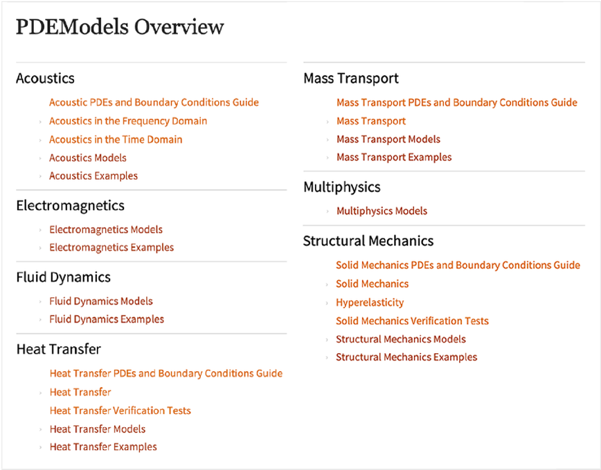
It’s all about providing symbolic “construction kits” for PDEs and their boundary conditions. We started this about five years ago, progressively covering more and more application areas. In Version 14 we’ve particularly focused on solid mechanics, fluid mechanics, electromagnetics and (one-particle) quantum mechanics.

Here’s an example from solid mechanics. First, we define the variables we’re dealing with (displacement and underlying coordinates):

Next, we specify the parameters we want to use to describe the solid material we’re going to work with:

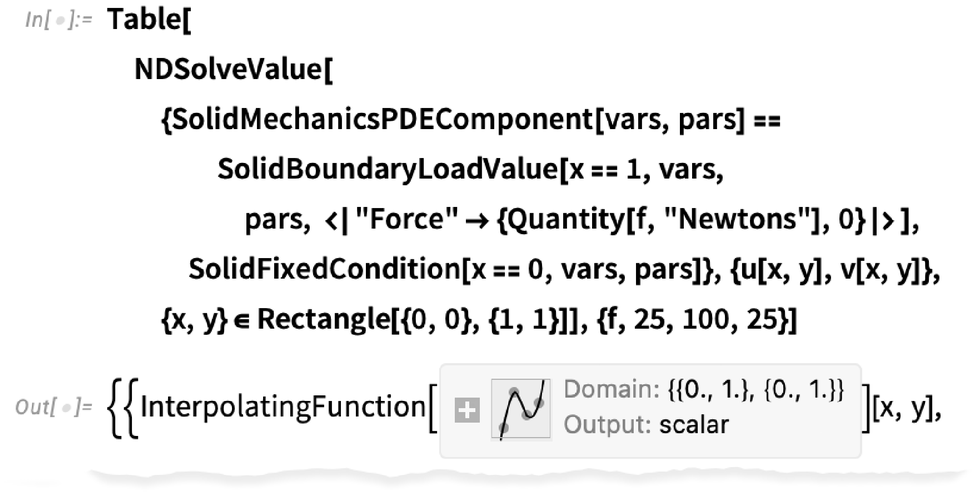
Now we can actually set up our PDE—using symbolic PDE specifications like SolidMechanicsPDEComponent—here for the deformation of a solid object pulled on one side:

And, yes, “underneath”, these simple symbolic specifications turn into a complicated “raw” PDE:
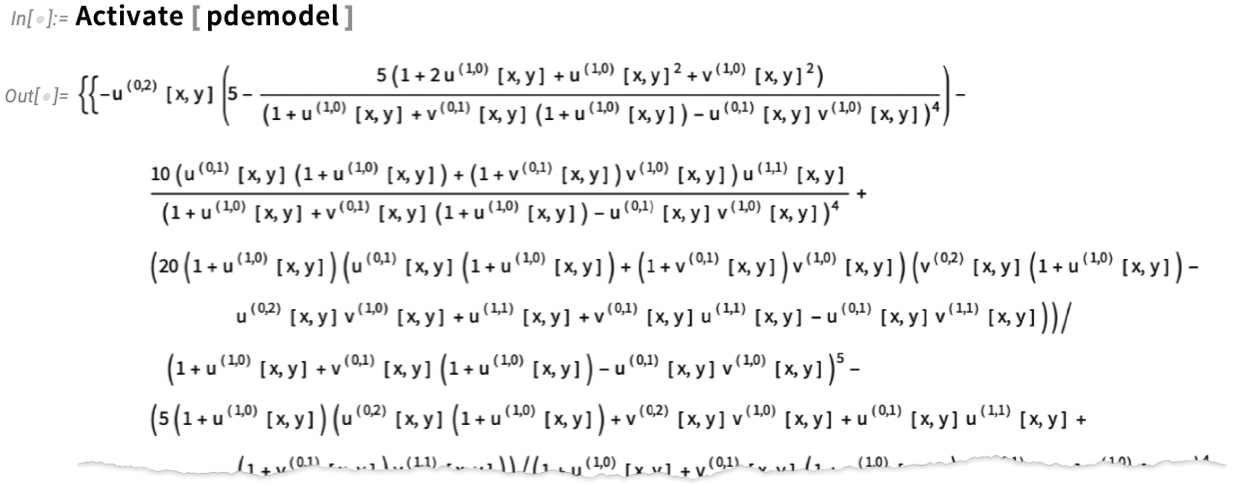
Now we are ready to actually solve our PDE in a particular region, i.e. for an object with a particular shape:
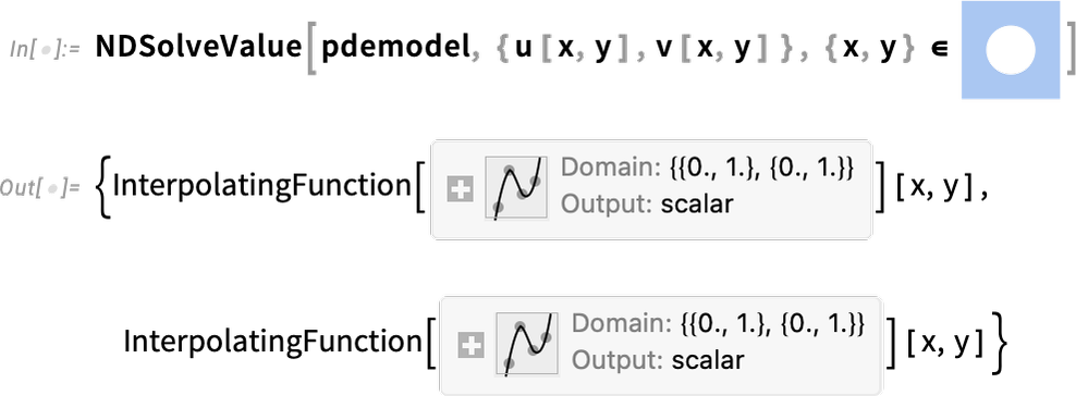
And now we can visualize the result, which shows how our object stretches when it’s pulled on:
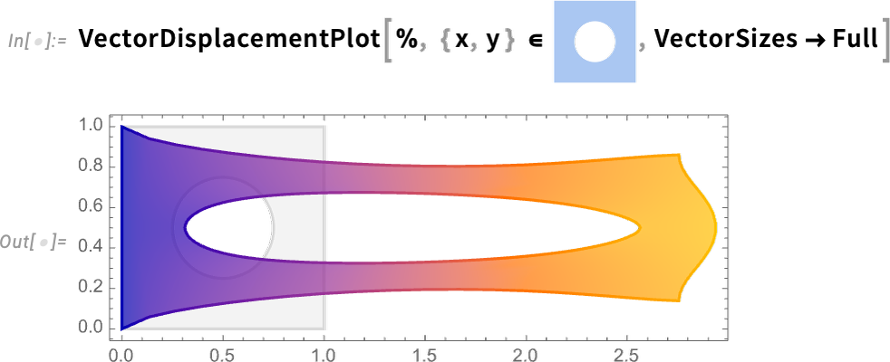
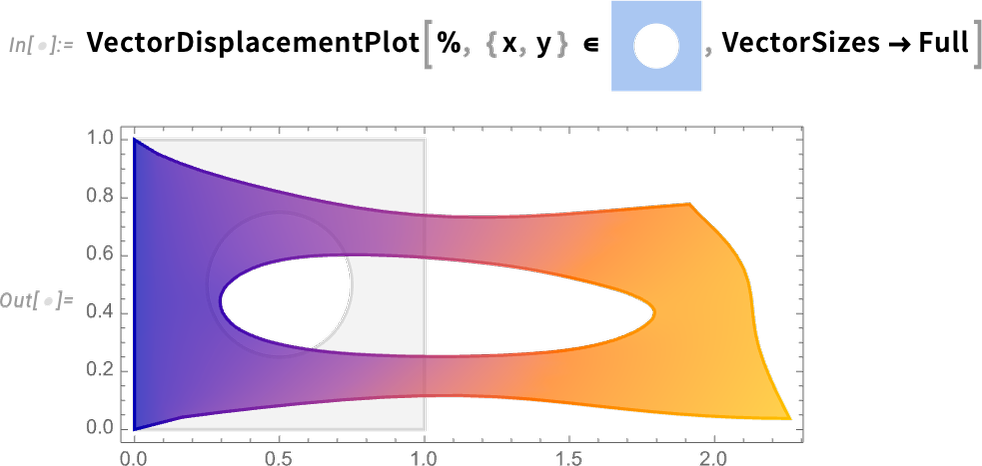
The way we’ve set things up, the material for our object is an idealization of something like rubber. But in the Wolfram Language we now have ways to specify all sorts of detailed properties of materials. So, for example, we can add reinforcement as a unit vector in a particular direction (say in practice with fibers) to our material:

Then we can rerun what we did before


but now we get a slightly different result:
Another major PDE domain that’s new in Version 14.0 is fluid flow. Let’s do a 2D example. Our variables are 2D velocity and pressure:

Now we can set up our fluid system in a particular region, with no-slip conditions on all walls except at the top where we assume fluid is flowing from left to right. The only parameter needed is the Reynolds number. And instead of just solving our PDEs for a single Reynolds number, let’s create a parametric solver that can take any specified Reynolds number:
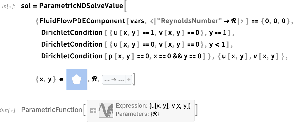
Now here’s the result for Reynolds number 100:
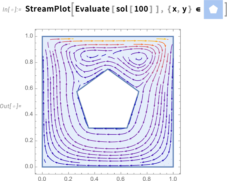
But with the way we’ve set things up, we can as well generate a whole video as a function of Reynolds number (and, yes, the Parallelize speeds things up by generating different frames in parallel):


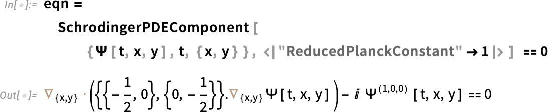
Much of our work in PDEs involves catering to the complexities of real-world engineering situations. But in Version 14.0 we’re also adding features to support “pure physics”, and in particular to support quantum mechanics done with the Schrödinger equation. So here, for example, is the 2D 1-particle Schrödinger equation (with ):

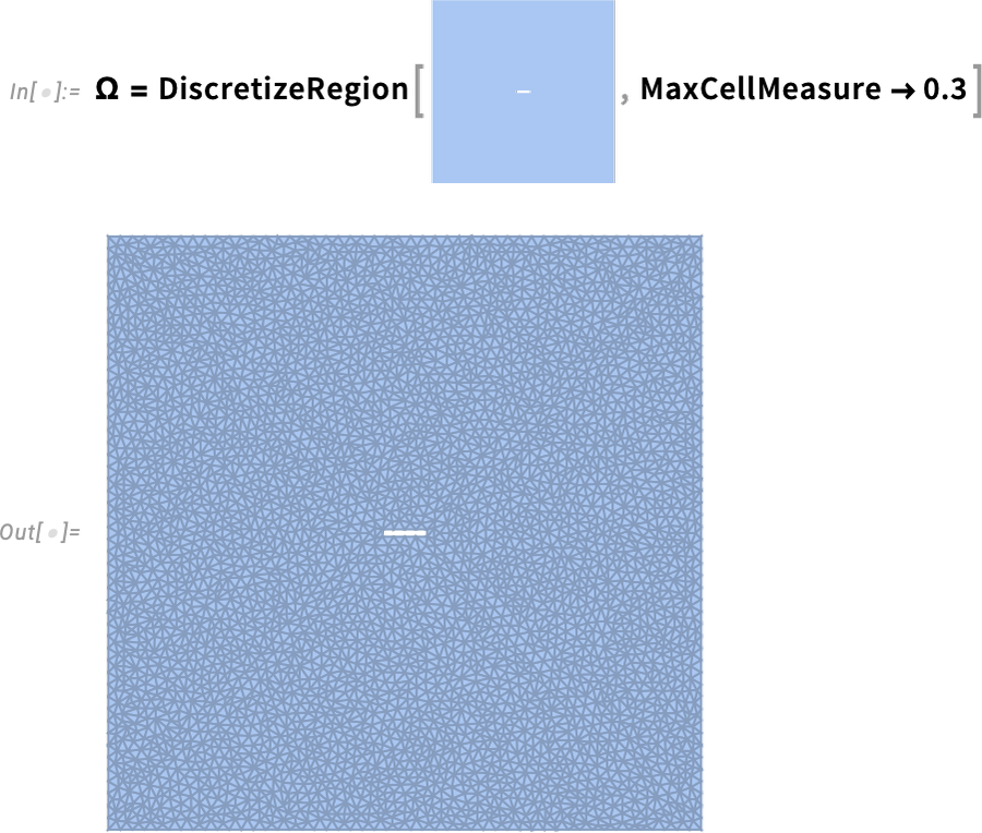
Here’s the region we’re going to be solving over—showing explicit discretization:
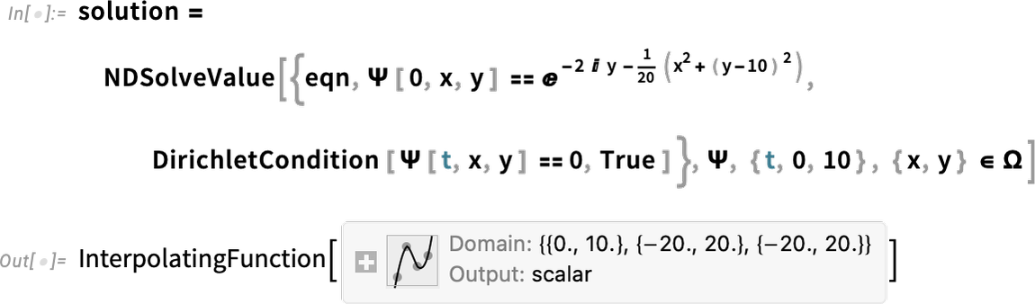
Now we can solve the equation, adding in some boundary conditions:
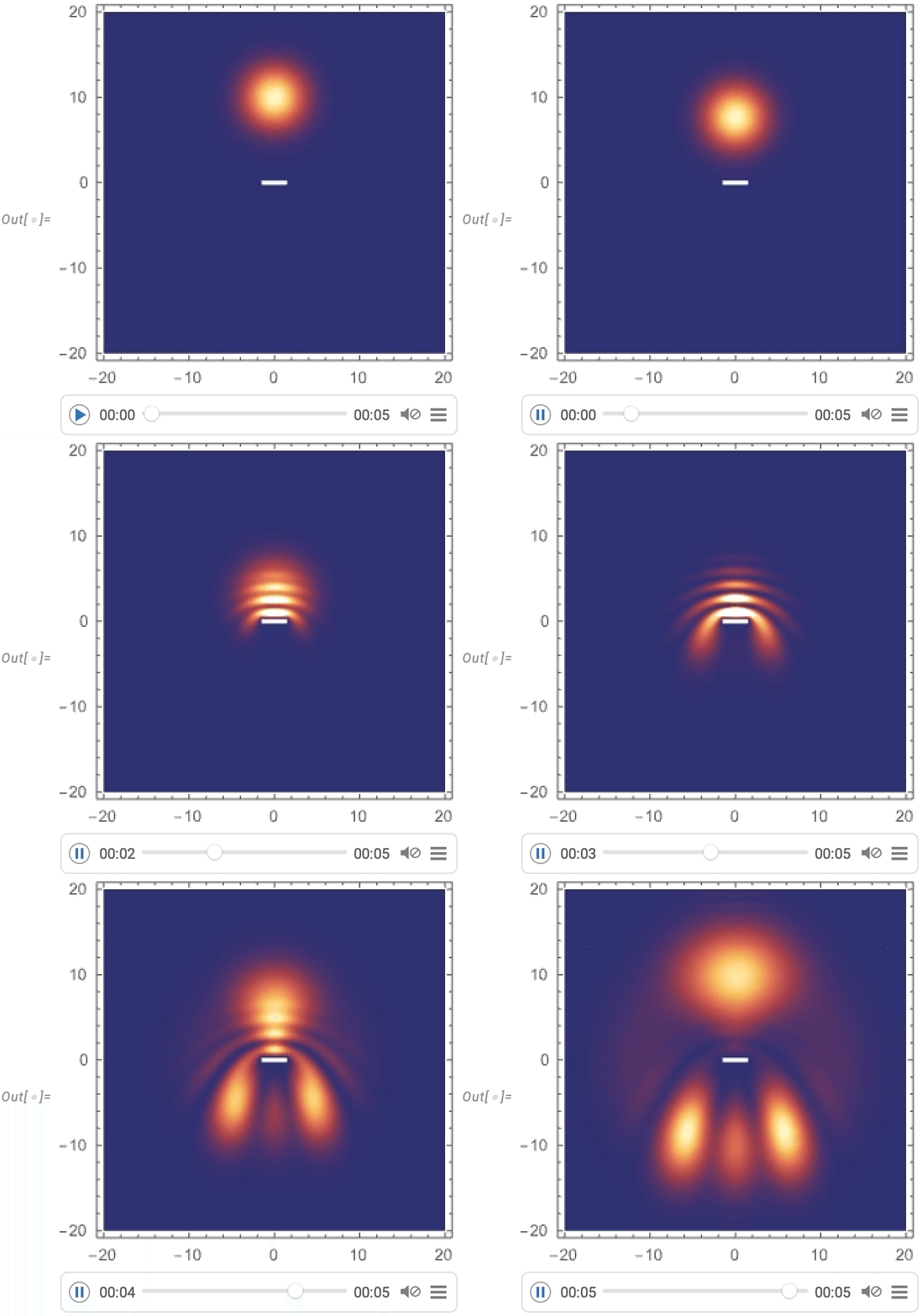
And now we get to visualize a Gaussian wave packet scattering around a barrier:

Streamlining Systems Engineering Computation

Systems engineering is a big field, but it’s one where the structure and capabilities of the Wolfram Language provide unique advantages—that over the past decade have allowed us to build out rather complete industrial-strength support for modeling, analysis and control design for a wide range of types of systems. It’s all an integrated part of the Wolfram Language, accessible through the computational and interface structure of the language. But it’s also integrated with our separate Wolfram System Modeler product, that provides a GUI-based workflow for system modeling and exploration.

Shared with System Modeler are large collections of domain-specific modeling libraries. And, for example, since Version 13, we’ve added libraries in areas such as battery engineering, hydraulic engineering and aircraft engineering—as well as educational libraries for mechanical engineering, thermal engineering, digital electronics, and biology. (We’ve also added libraries for areas such as business and public policy simulation.)

Domain-specific modeling libraries

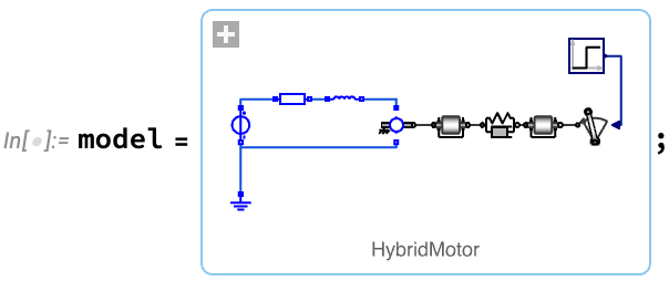
A typical workflow for systems engineering begins with the setting up of a model. The model can be built from scratch, or assembled from components in model libraries—either visually in Wolfram System Modeler, or programmatically in the Wolfram Language. For example, here’s a model of an electric motor that’s turning a load through a flexible shaft:
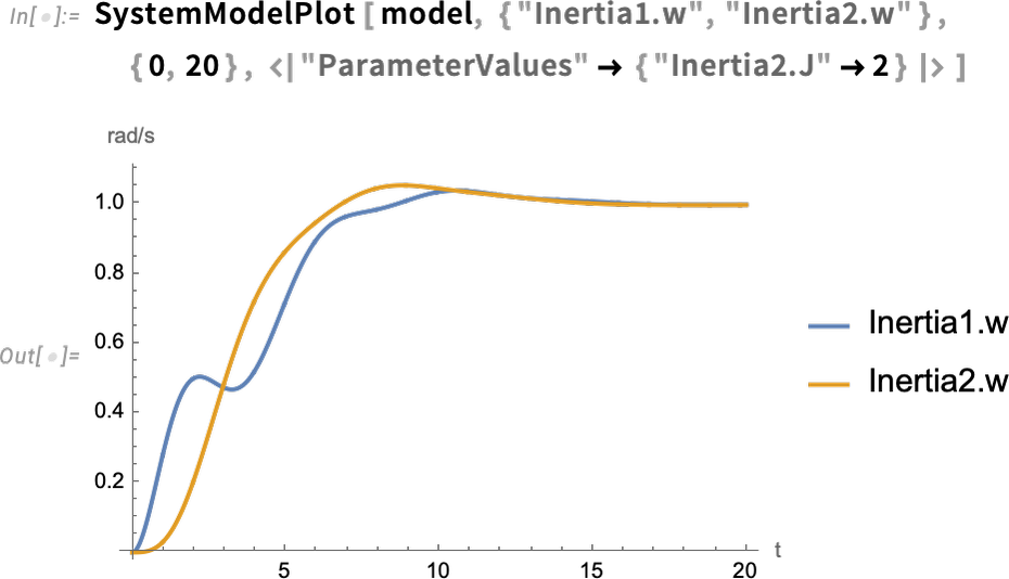
Once one’s got a model, one can then simulate it. Here’s an example where we’ve set one parameter of our model (the moment of inertia of the load), and we’re computing the values of two others as a function of time:
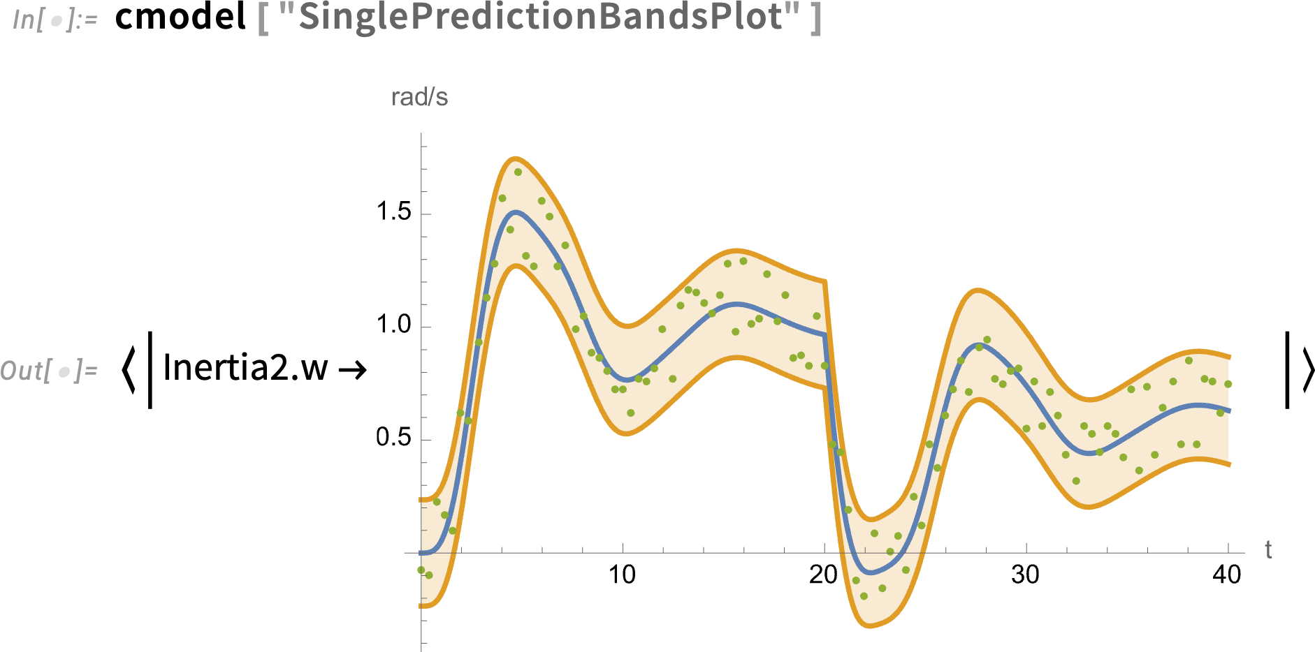
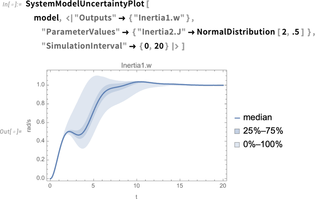
A new capability in Version 14.0 is being able to see the effect of uncertainty in parameters (or initial values, etc.) on the behavior of a system. So here, as an example, we’re saying the value of the parameter is not definite, but is instead distributed according to a normal distribution—then we’re seeing the distribution of output results:
The motor with flexible shaft that we’re looking at can be thought of as a “multidomain system”, combining electrical and mechanical components. But the Wolfram Language (and Wolfram System Modeler) can also handle “mixed systems”, combining analog and digital (i.e. continuous and discrete) components. Here’s a fairly sophisticated example from the world of control systems: a helicopter model connected in a closed loop to a digital control system:

Helicopter model

This whole model system can be represented symbolically just by:

And now we compute the input-output response of the model:

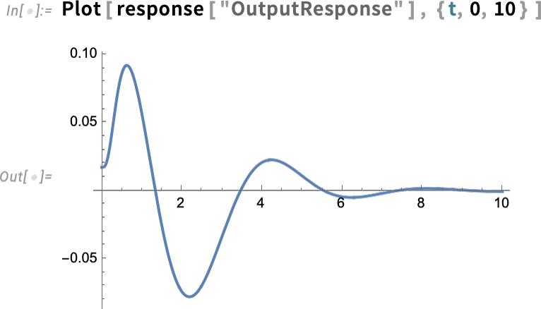
Here’s specifically the output response:
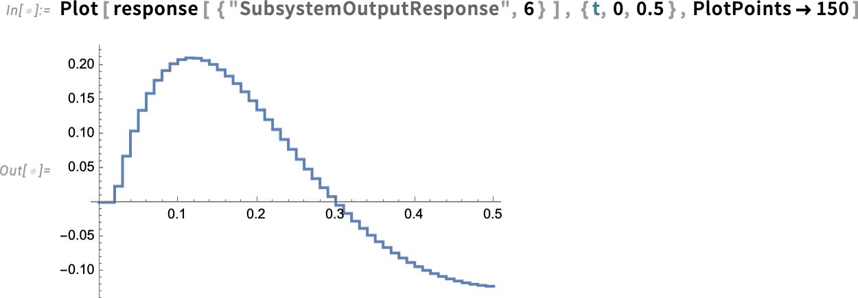
But now we can “drill in” and see specific subsystem responses, here of the zero-order hold device (labeled ZOH above)—complete with its little digital steps:
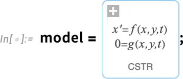
But what if we want to design the control systems ourselves? Well, in Version 14 we can now apply all our Wolfram Language control systems design functionality to arbitrary system models. Here’s an example of a simple model, in this case in chemical engineering (a continuously stirred tank):
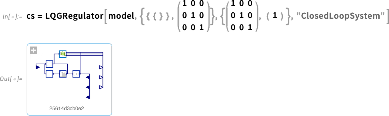
Now we can take this model and design an LQG controller for it—then assemble a whole closed-loop system for it:
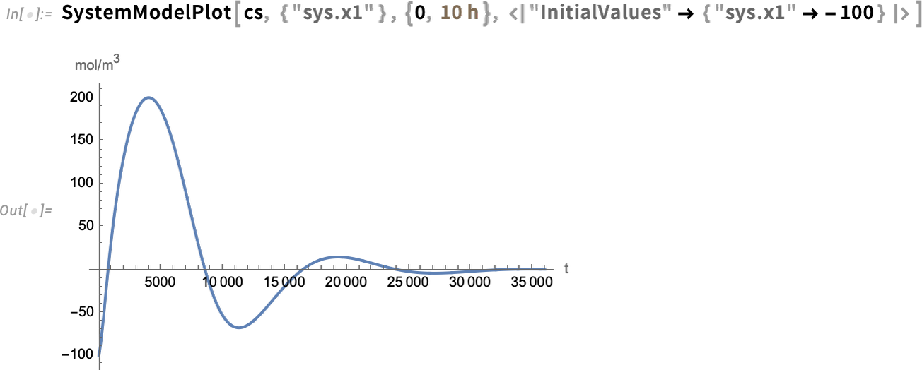
Now we can simulate the closed-loop system—and see that the controller succeeds in bringing the final value to 0:
Graphics: More Beautiful & Alive

Graphics have always been an important part of the story of the Wolfram Language, and for more than three decades we’ve been progressively enhancing and updating their appearance and functionality—sometimes with help from advances in hardware (e.g. GPU) capabilities.

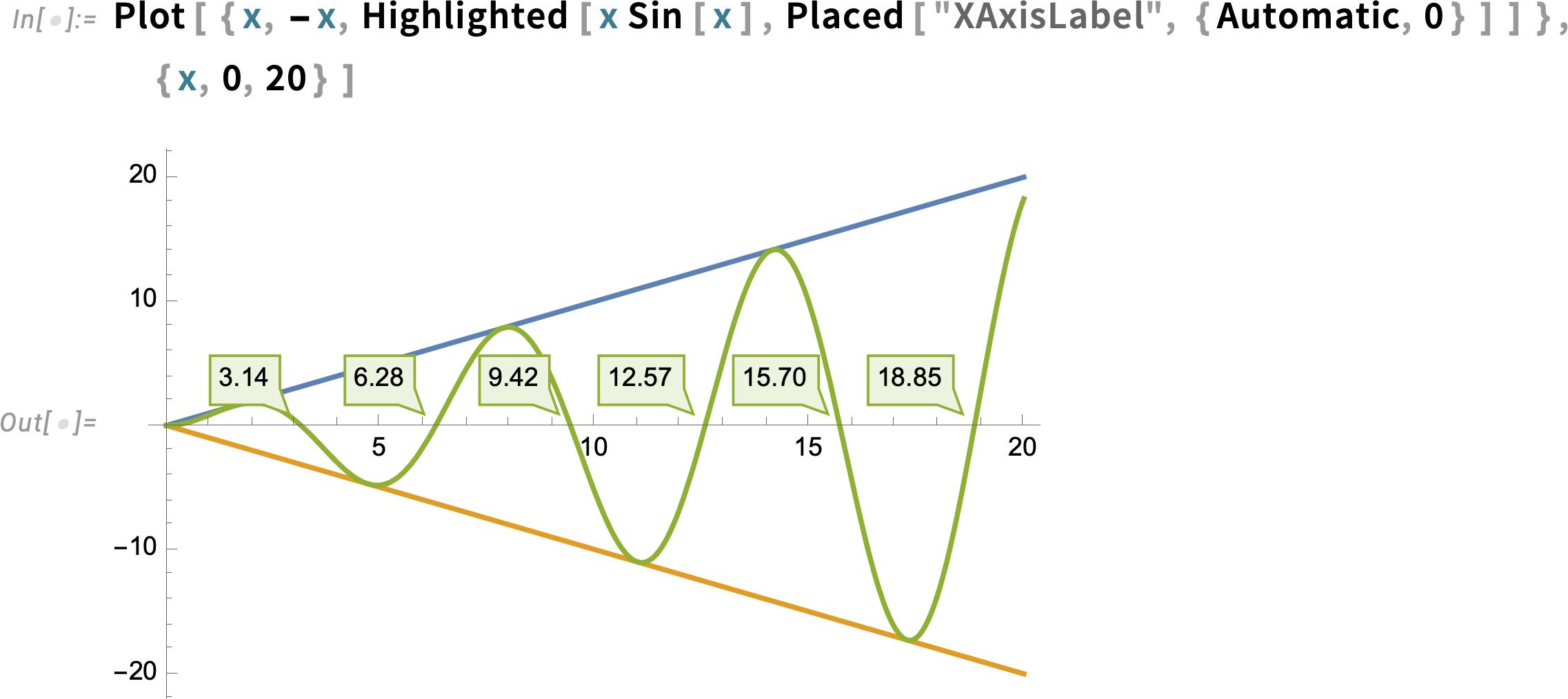
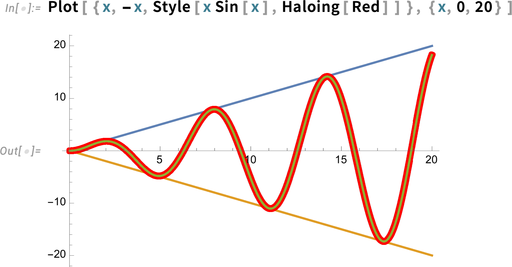
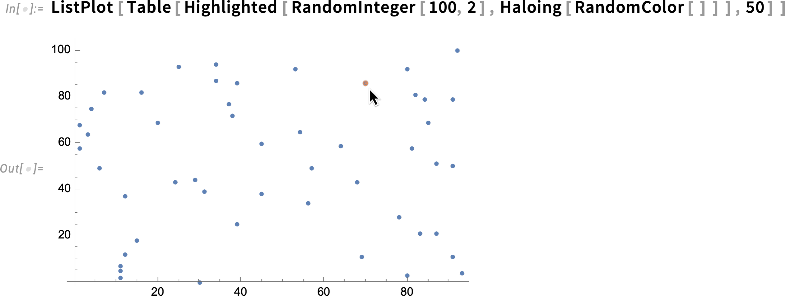
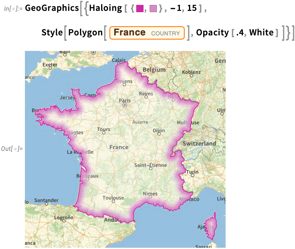
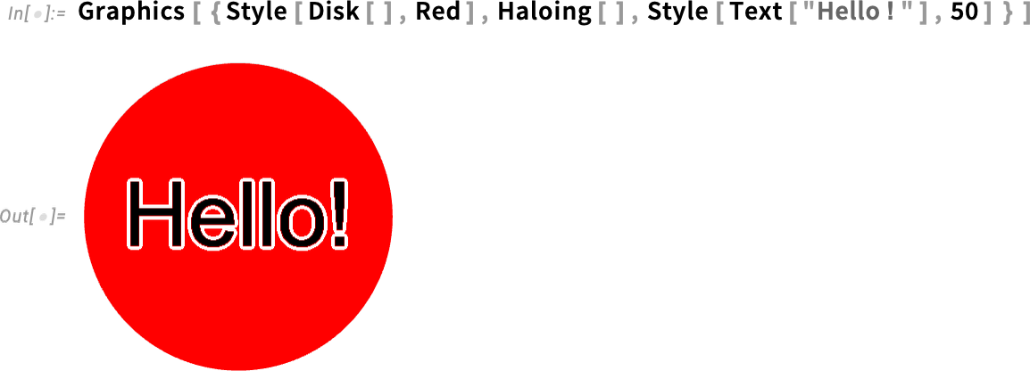
Since Version 13 we’ve added a variety of “decorative” (or “annotative”) effects in 2D graphics. One example (useful for putting captions on things) is Haloing:
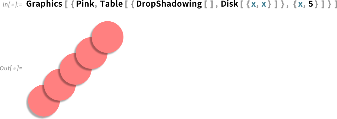
Another example is DropShadowing:
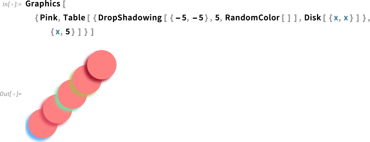
All of these are specified symbolically, and can be used throughout the system (e.g. in hover effects, etc). And, yes, there are many detailed parameters you can set:
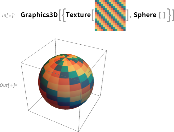
A significant new capability in Version 14.0 is convenient texture mapping. We’ve had low-level polygon-by-polygon textures for a decade and a half. But now in Version 14.0 we’ve made it straightforward to map textures onto whole surfaces. Here’s an example wrapping a texture onto a sphere:
And here’s wrapping the same texture onto a more complicated surface:
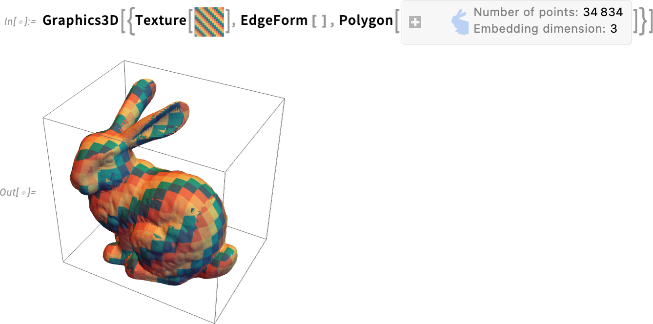
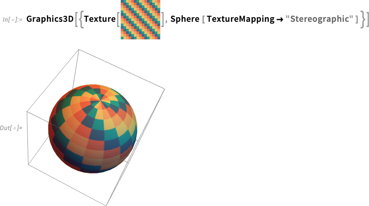
A significant subtlety is that there are many ways to map what amount to “texture coordinate patches” onto surfaces. The documentation illustrates new, named cases:

Texture coordinate patches

And now here’s what happens with stereographic projection onto a sphere:
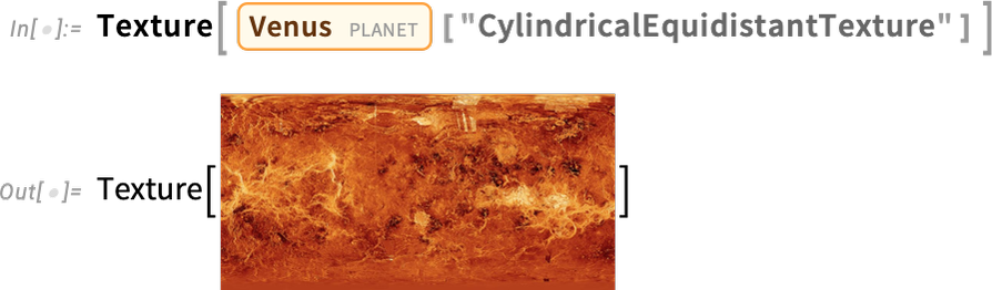
Here’s an example of “surface texture” for the planet Venus
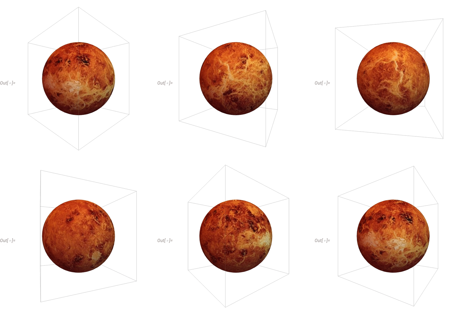
and here it’s been mapped onto a sphere, which can be rotated:

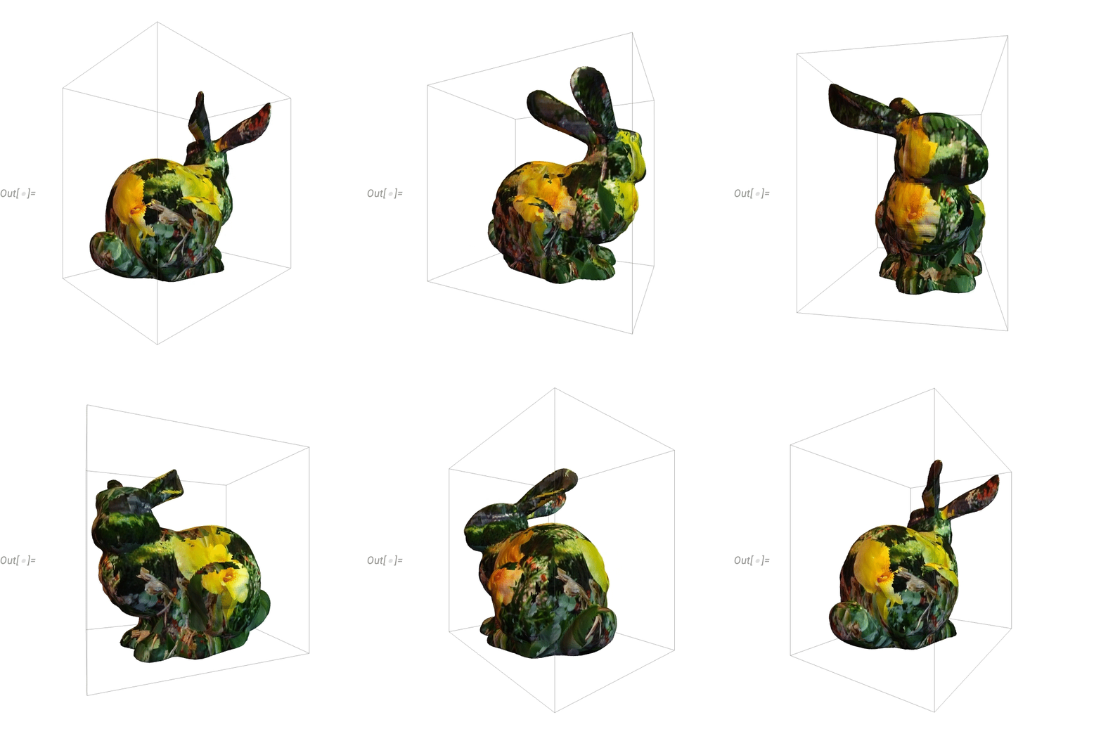
Here’s a “flowerified” bunny:
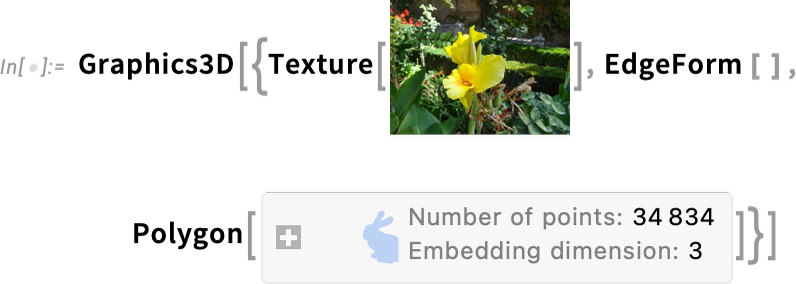
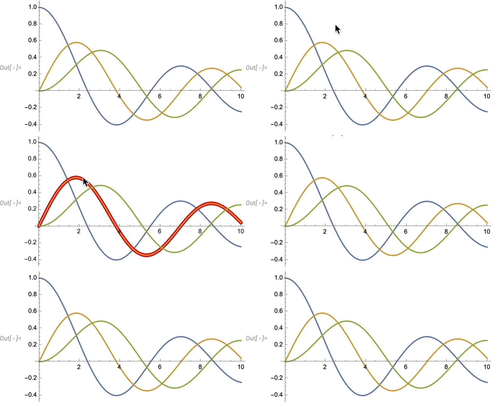
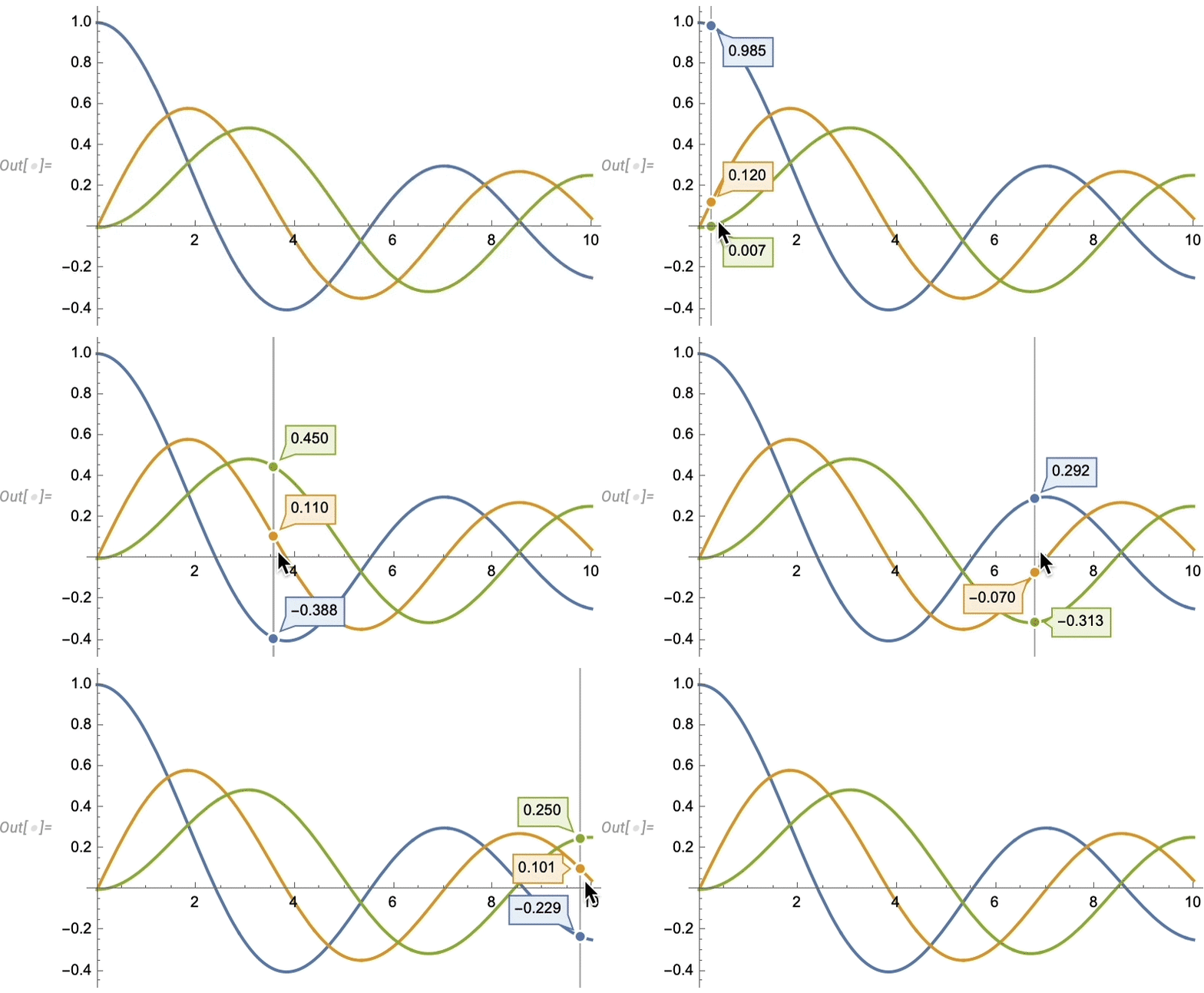
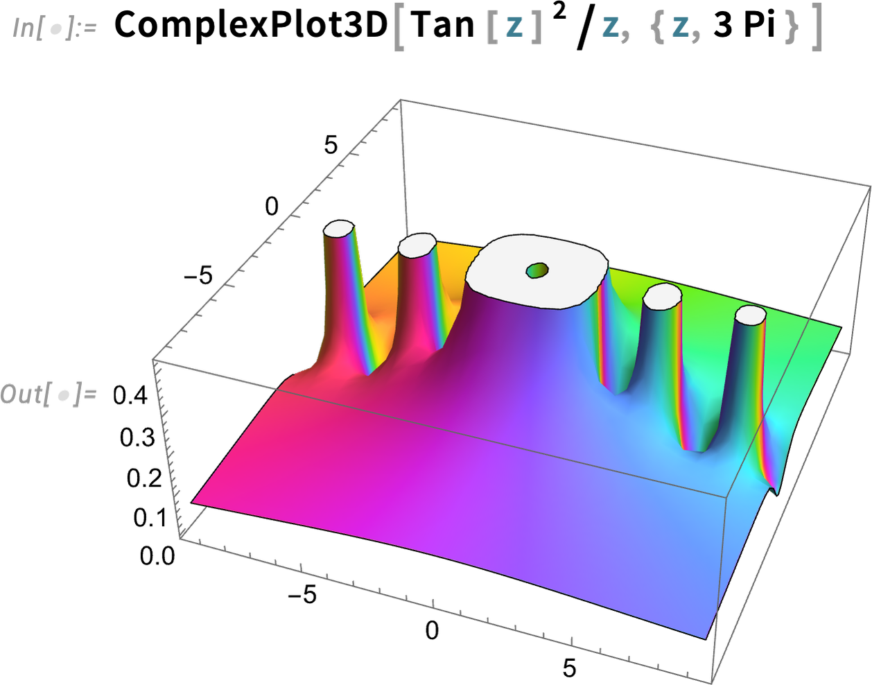
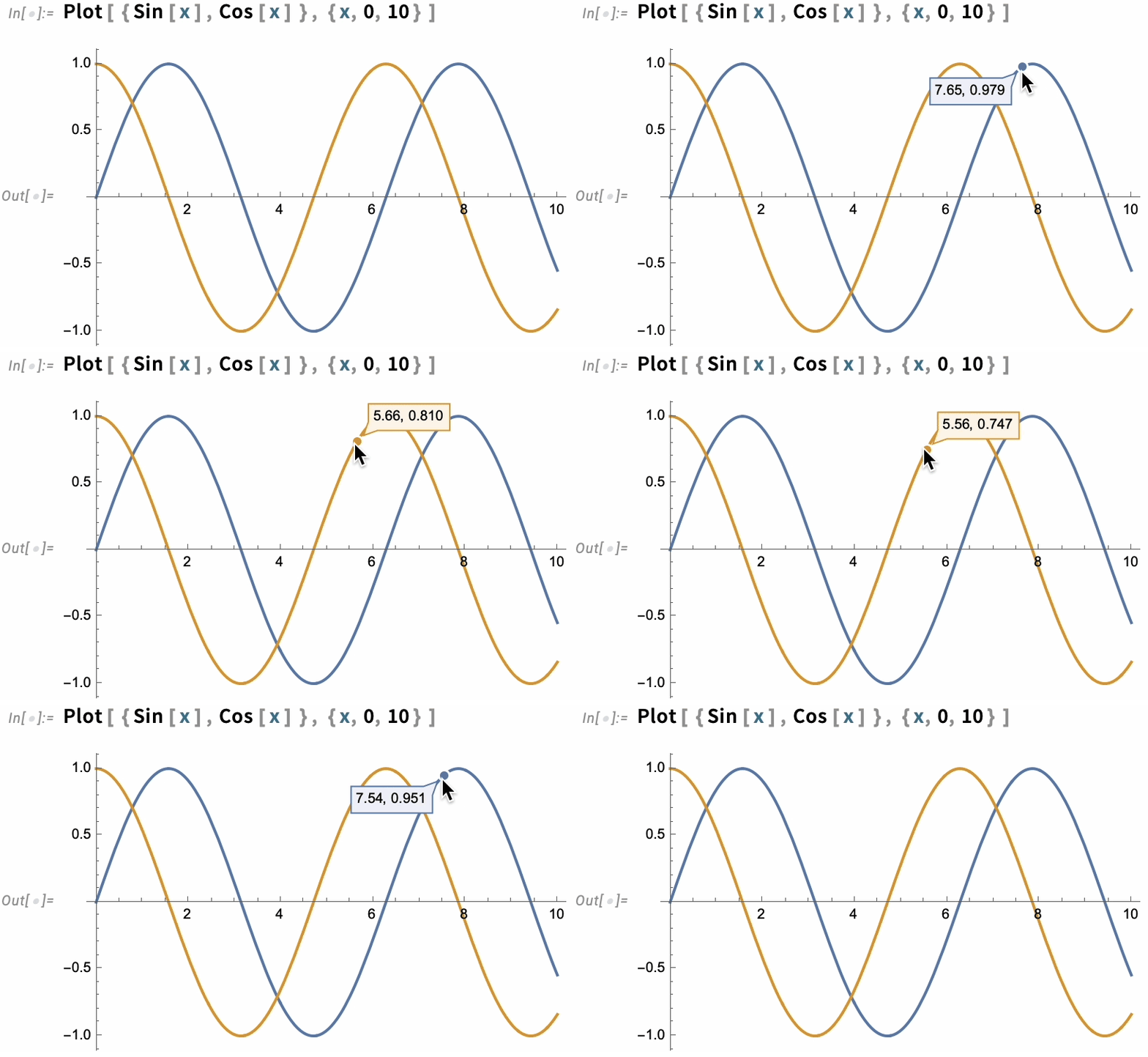
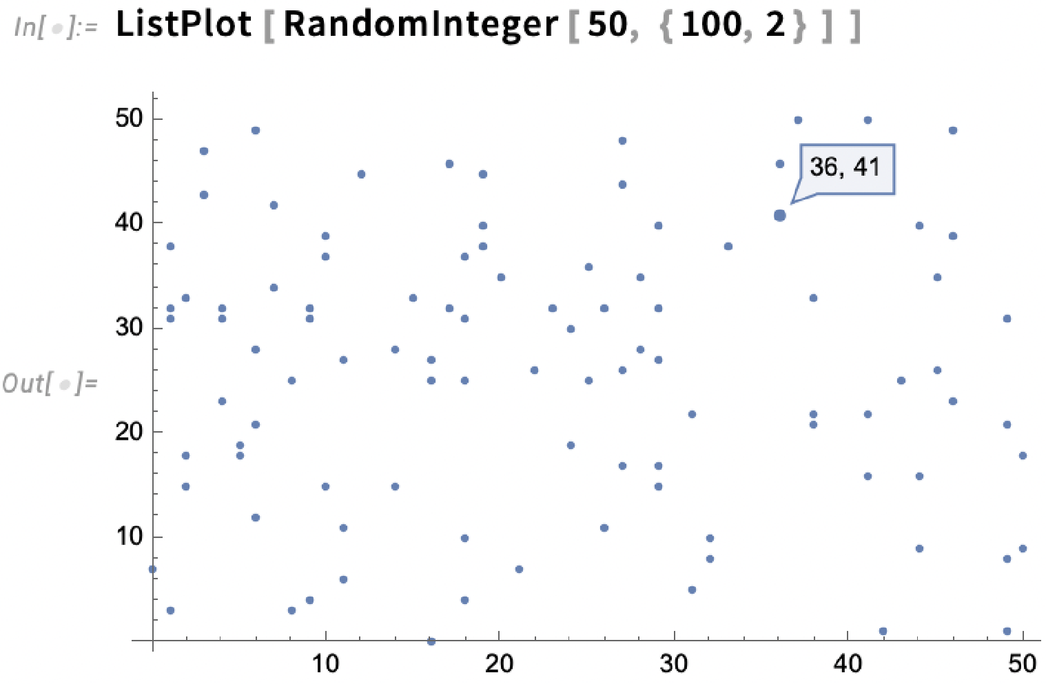
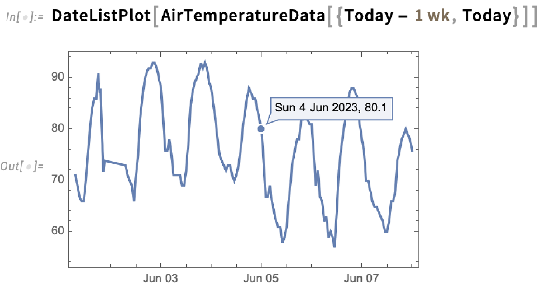
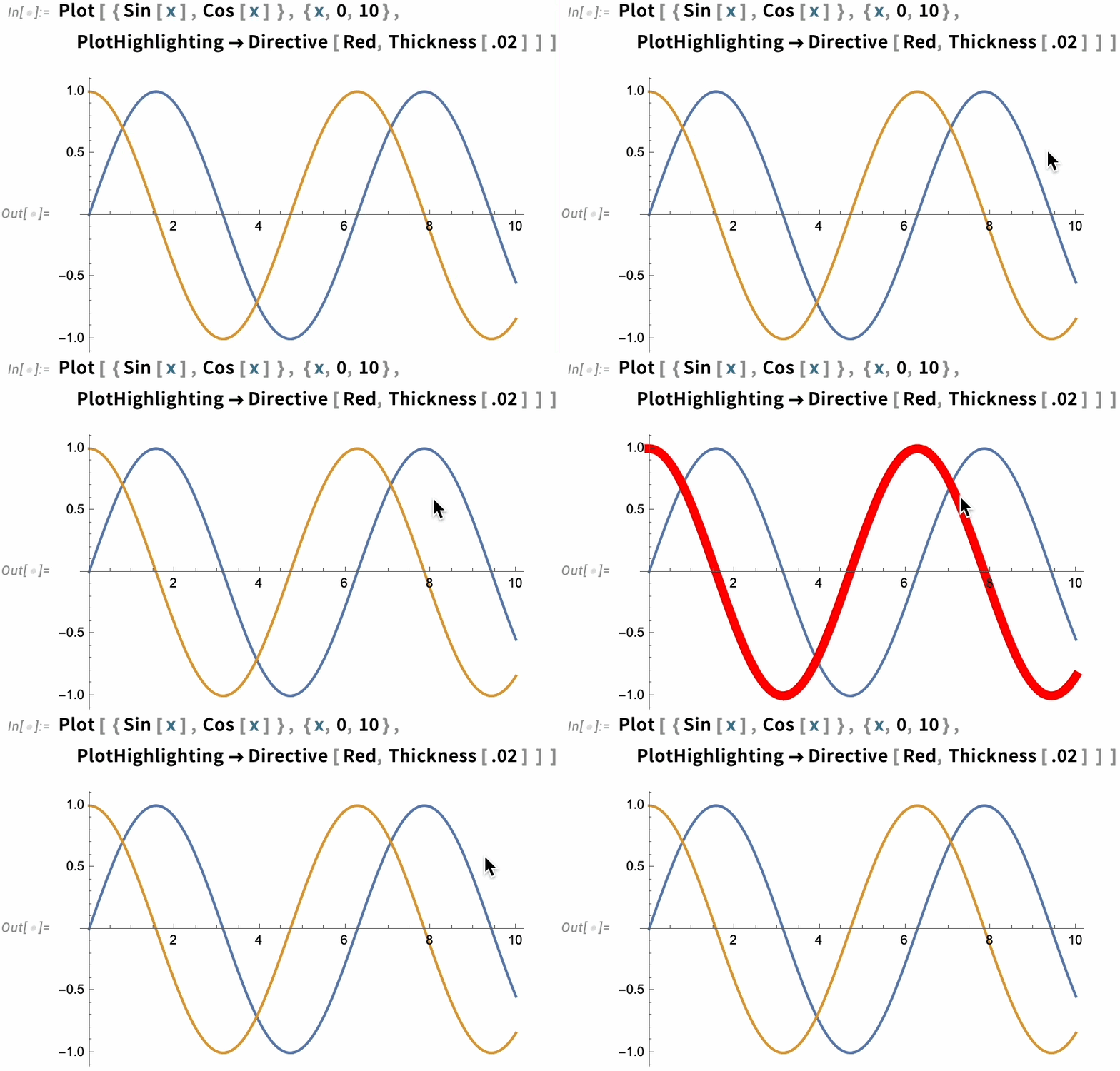
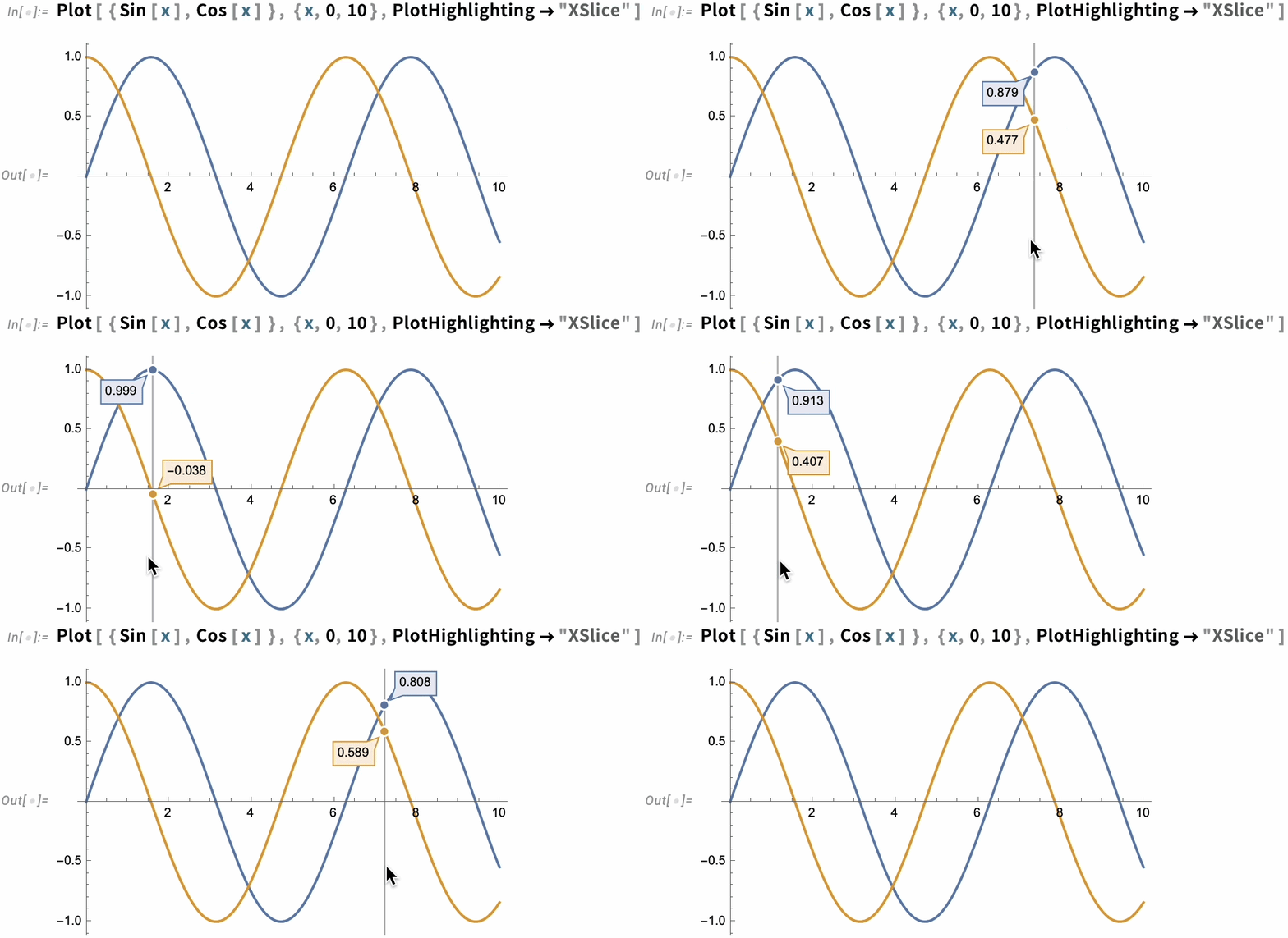
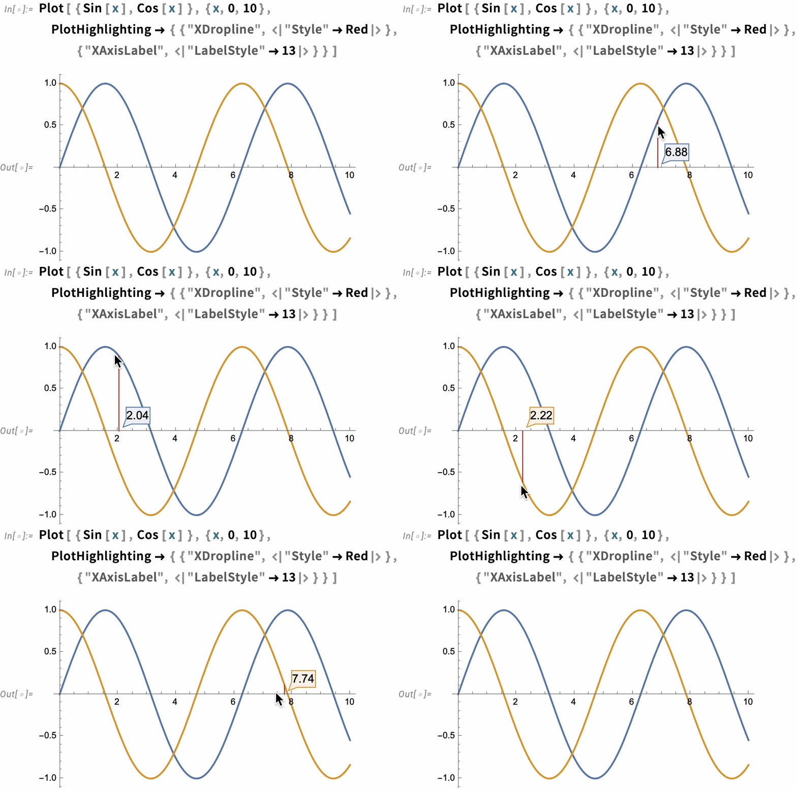
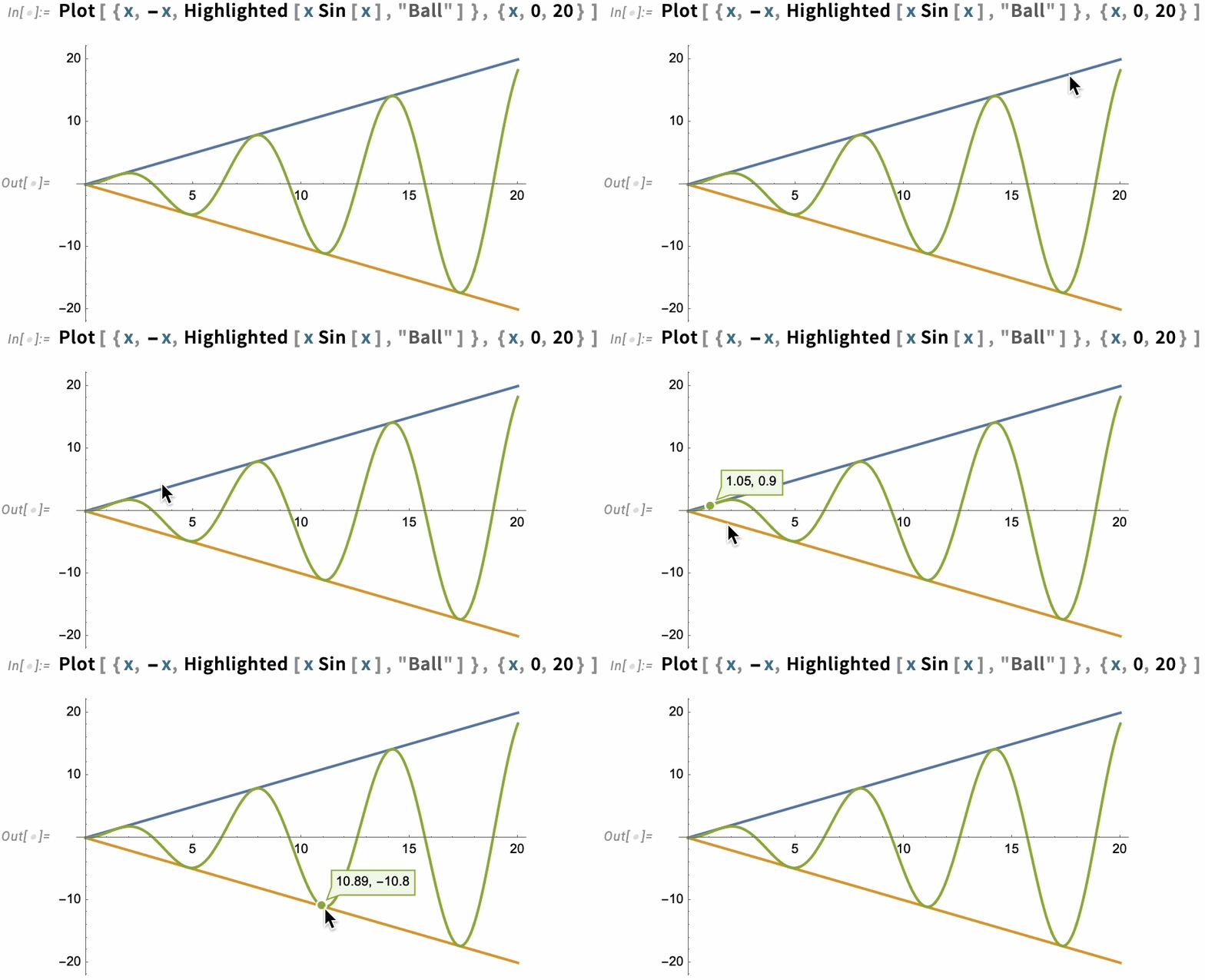
Things like texture mapping help make graphics visually compelling. Since Version 13 we’ve also added a variety of “live visualization” capabilities that automatically “bring visualizations to life”. For example, any plot now by default has a “coordinate mouseover”:

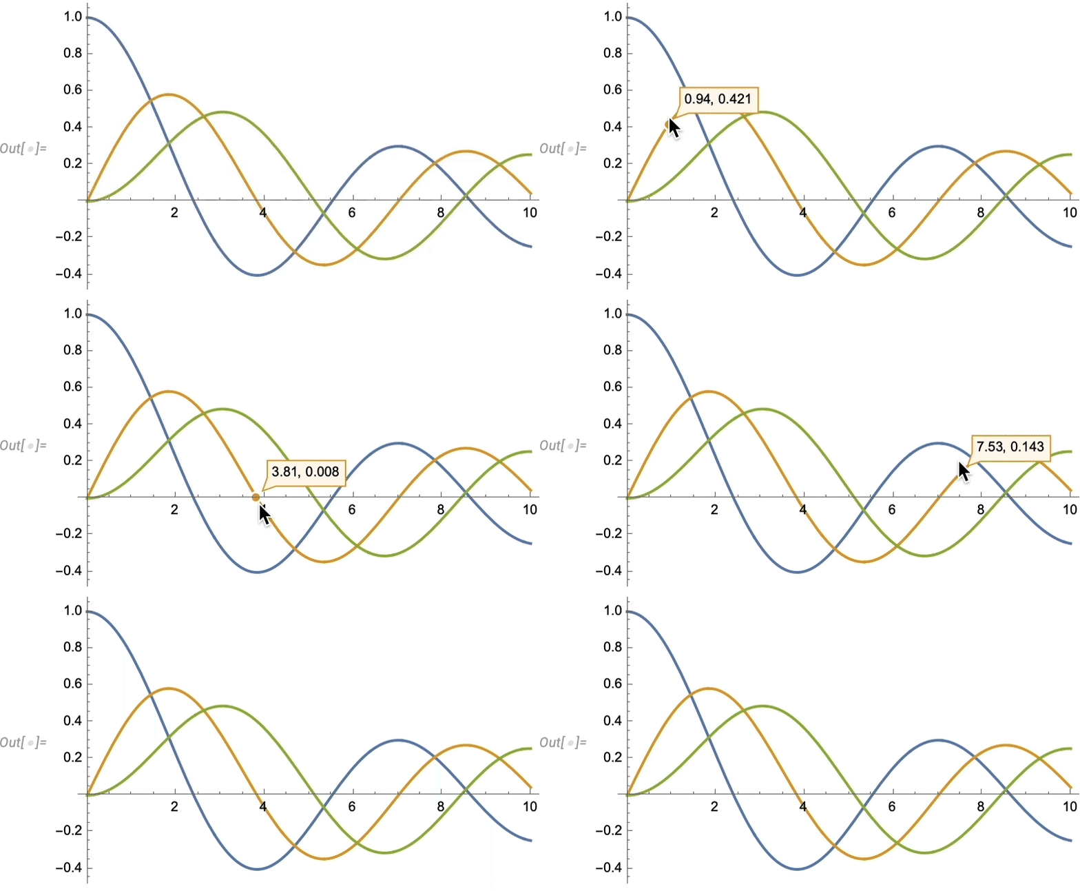
As usual, there’s lots of ways to control such “highlighting” effects:

Euclid Redux: The Advance of Synthetic Geometry

One might say it’s been two thousand years in the making. But four years ago (Version 12) we began to introduce a computable version of Euclid-style synthetic geometry.

The idea is to specify geometric scenes symbolically by giving a collection of (potentially implicit) constraints:

We can then generate a random instance of geometry consistent with the constraints—and in Version 14 we’ve considerably enhanced our ability to make sure that geometry will be “typical” and non-degenerate:

But now a new feature of Version 14 is that we can find values of geometric quantities that are determined by the constraints:

Here’s a slightly more complicated case:

And here we’re now solving for the areas of two triangles in the figure:

We’ve always been able to give explicit styles for particular elements of a scene:
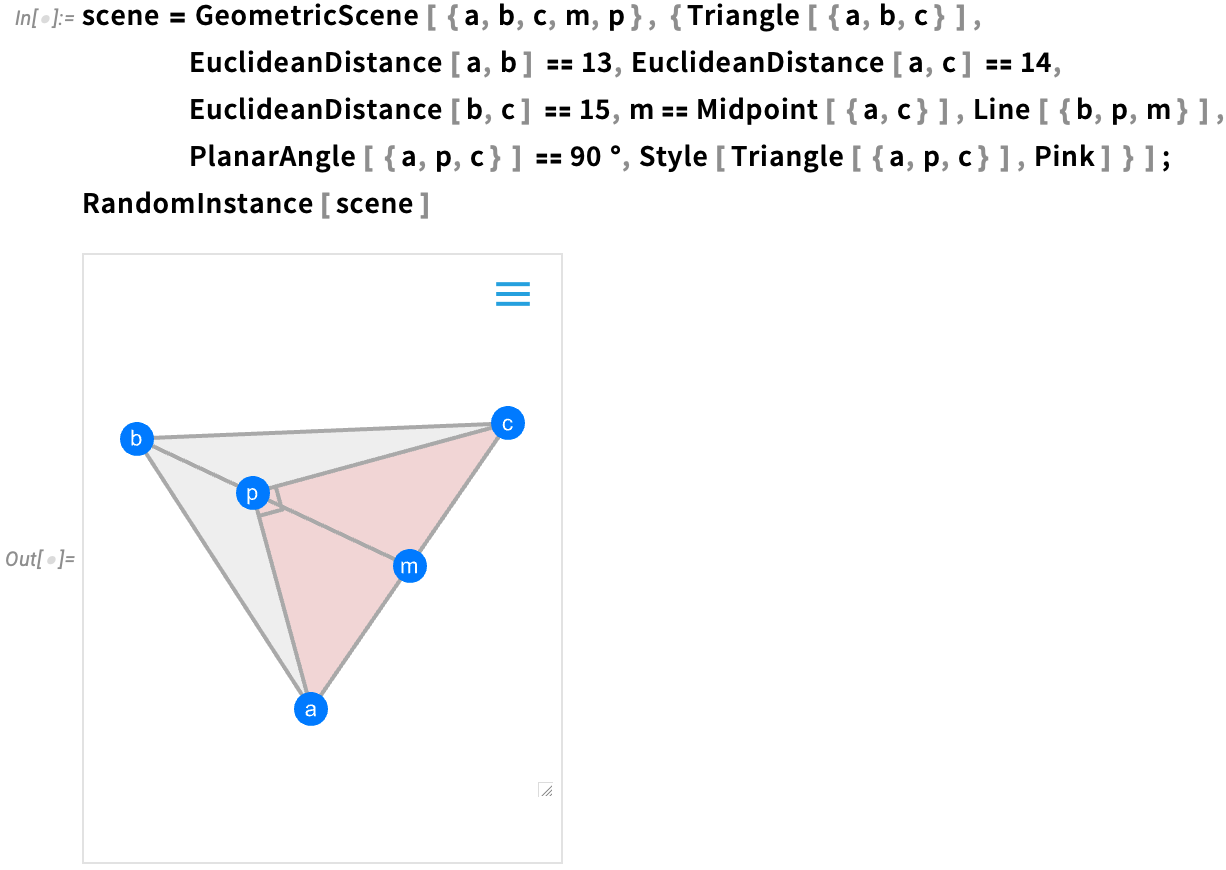
Now one of the new features in Version 14 is being able to give general “geometric styling rules”, here just assigning random colors to each element:

The Ever-Smoother User Interface

Our goal with Wolfram Language is to make it as easy as possible to express oneself computationally. And a big part of achieving that is the coherent design of the language itself. But there’s another part as well, which is being able to actually enter Wolfram Language input one wants—say in a notebook—as easily as possible. And with every new version we make enhancements to this.

One area that’s been in continuous development is interactive syntax highlighting. We first added syntax highlighting nearly two decades ago—and over time we’ve progressively made it more and more sophisticated, responding both as you type, and as code gets executed. Some highlighting has always had obvious meaning. But particularly highlighting that is dynamic and based on cursor position has sometimes been harder to interpret. And in Version 14—leveraging the brighter color palettes that have become the norm in recent years—we’ve tuned our dynamic highlighting so it’s easier to quickly tell “where you are” within the structure of an expression:

Dynamic highlighting

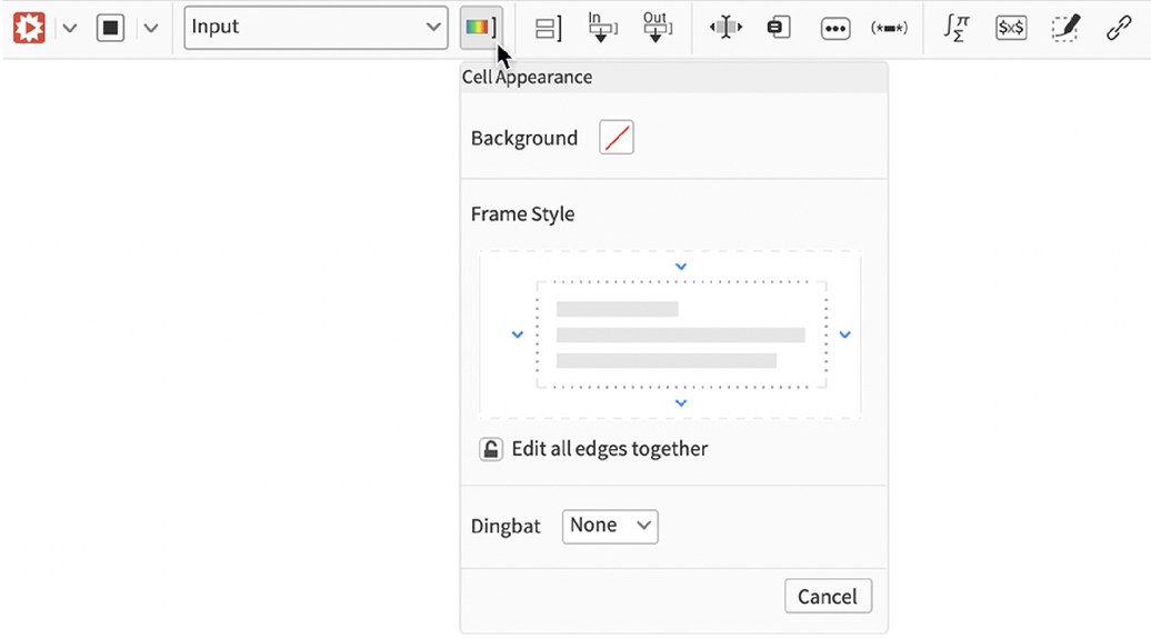
On the subject of “knowing what one has”, another enhancement—added in Version 13.2—is differentiated frame coloring for different kinds of visual objects in notebooks. Is that thing one has a graphic? Or an image? Or a graph? Now one can tell from the color of frame when one selects it:

Differentiated frame coloring

An important aspect of the Wolfram Language is that the names of built-in functions are spelled out enough that it’s easy to tell what they do. But often the names are therefore necessarily quite long, and so it’s important to be able to autocomplete them when one’s typing. In 13.3 we added the notion of “fuzzy autocompletion” that not only “completes to the end” a name one’s typing, but also can fill in intermediate letters, change capitalization, etc. Thus, for example, just typing lll brings up an autocompletion menu that begins with ListLogLogPlot:

Autocompletion menu

A major user interface update that first appeared in Version 13.1—and has been enhanced in subsequent versions—is a default toolbar for every notebook:

Default toolbar

The toolbar provides immediate access to evaluation controls, cell formatting and various kinds of input (like inline cells, , hyperlinks, drawing canvas, etc.)—as well as to things like Menu options cloud publishing, Menu options documentation search and Menu options “chat” (i.e. LLM) settings.

Much of the time, it’s useful to have the toolbar displayed in any notebook you’re working with. But on the left-hand side there’s a little tiny that lets you minimize the toolbar:

Minimize toolbar

In 14.0 there’s a Preferences setting that makes the toolbar come up minimized in any new notebook you create—and this in effect gives you the best of both worlds: you have immediate access to the toolbar, but your notebooks don’t have anything “extra” that might distract from their content.

Another thing that’s advanced since Version 13 is the handling of “summary” forms of output in notebooks. A basic example is what happens if you generate a very large result. By default only a summary of the result is actually displayed. But now there’s a bar at the bottom that gives various options for how to handle the actual output:

By default, the output is only stored in your current kernel session. But by pressing the Iconize button you get an iconized form that will appear directly in your notebook (or one that can be copied anywhere) and that “has the whole output inside”. There’s also a Store full expression in notebook button, which will “invisibly” store the output expression “behind” the summary display.

If the expression is stored in the notebook, then it’ll be persistent across kernel sessions. Otherwise, well, you won’t be able to get to it in a different kernel session; the only thing you’ll have is the summary display:

Summary display

It’s a similar story for large “computational objects”. Like here’s a Nearest function with a million data points:
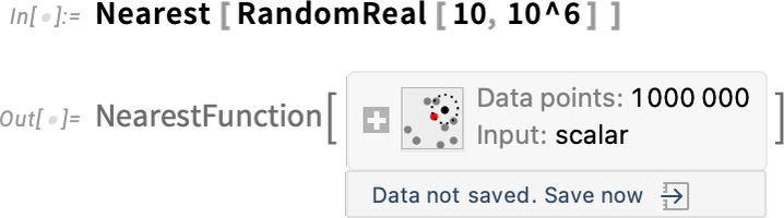
By default, the data is just something that exists in your current kernel session. But now there’s a menu that lets you save the data in various persistent locations:

Save data menu

And There’s the Cloud Too

There are many ways to run the Wolfram Language. Even in Version 1.0 we had the notion of remote kernels: the notebook front end running on one machine (in those days essentially always a Mac, or a NeXT), and the kernel running on a different machine (in those days sometimes even connected by phone lines). But a decade ago came a major step forward: the Wolfram Cloud.

There are really two distinct ways in which the cloud is used. The first is in delivering a notebook experience similar to our longtime desktop experience, but running purely in a browser. And the second is in delivering APIs and other programmatically accessed capabilities—notably, even at the beginning, a decade ago, through things like APIFunction.

The Wolfram Cloud has been the target of intense development now for nearly 15 years. Alongside it have also come Wolfram Application Server and Wolfram Web Engine, which provide more streamlined support specifically for APIs (without things like user management, etc., but with things like clustering).

All of these—but particularly the Wolfram Cloud—have become core technology capabilities for us, supporting many of our other activities. So, for example, the Wolfram Function Repository and Wolfram Paclet Repository are both based on the Wolfram Cloud (and in fact this is true of our whole resource system). And when we came to build the Wolfram plugin for ChatGPT earlier this year, using the Wolfram Cloud allowed us to have the plugin deployed within a matter of days.

Since Version 13 there have been quite a few very different applications of the Wolfram Cloud. One is for the function ARPublish, which takes 3D geometry and puts it in the Wolfram Cloud with appropriate metadata to allow phones to get augmented-reality versions from a QR code of a cloud URL:
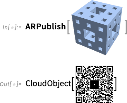
Augmented-reality triptych

On the Cloud Notebook side, there’s been a steady increase in usage, notably of embedded Cloud Notebooks, which have for example become common on Wolfram Community, and are used all over the Wolfram Demonstrations Project. Our goal all along has been to make Cloud Notebooks be as easy to use as simple webpages, but to have the depth of capabilities that we’ve developed in notebooks over the past 35 years. We achieved this some years ago for fairly small notebooks, but in the past couple of years we’ve been going progressively further in handling even multi-hundred-megabyte notebooks. It’s a complicated story of caching, refreshing—and dodging the vicissitudes of web browsers. But at this point the vast majority of notebooks can be seamlessly deployed to the cloud, and will display as immediately as simple webpages.

The Great Integration Story for External Code

It’s been possible to call external code from Wolfram Language ever since Version 1.0. But in Version 14 there are important advances in the extent and ease with which external code can be integrated. The overall goal is to be able to use all the power and coherence of the Wolfram Language even when some part of a computation is done in external code. And in Version 14 we’ve done a lot to streamline and automate the process by which external code can be integrated into the language.

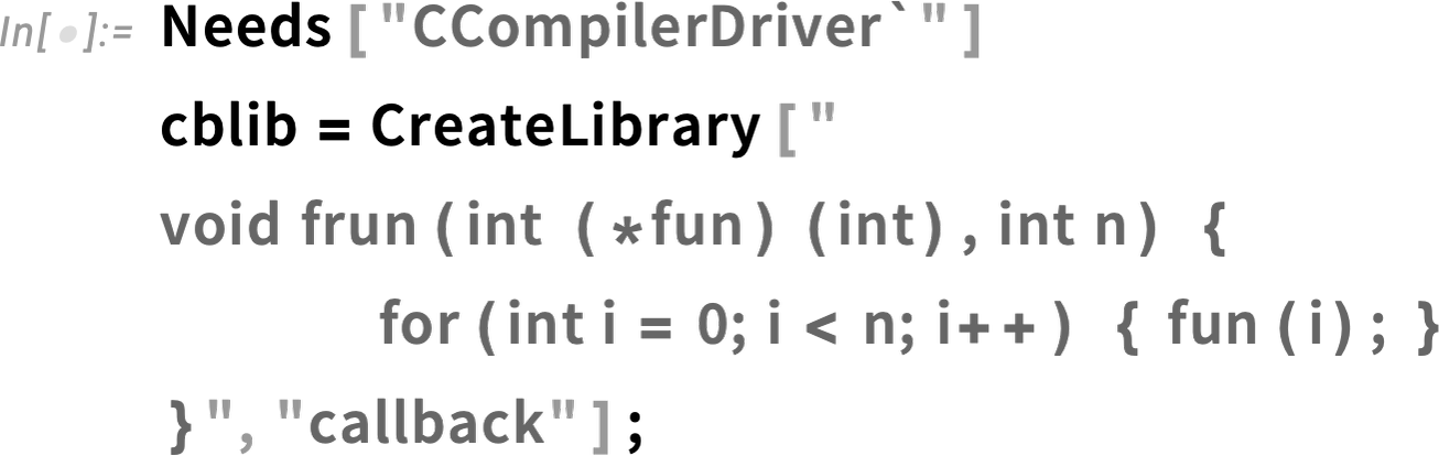
Once something is integrated into the Wolfram Language it just becomes, for example, a function that can be used just like any other Wolfram Language function. But what’s underneath is necessarily quite different for different kinds of external code. There’s one setup for interpreted languages like Python. There’s another for C-like compiled languages and dynamic libraries. (And then there are others for external processes, APIs, and what amount to “importable code specifications”, say for neural networks.)

Let’s start with Python. We’ve had ExternalEvaluate for evaluating Python code since 2018. But when you actually come to use Python there are all these dependencies and libraries to deal with. And, yes, that’s one of the places where the incredible advantages of the Wolfram Language and its coherent design are painfully evident. But in Version 14.0 we now have a way to encapsulate all that Python complexity, so that we can deliver Python functionality within Wolfram Language, hiding all the messiness of Python dependencies, and even the versioning of Python itself.

As an example, let’s say we want to make a Wolfram Language function Emojize that uses the Python function emojize within the emoji Python library. Here’s how we can do that:

And now you can just call Emojize in the Wolfram Language and—under the hood—it’ll run Python code:

The way this works is that the first time you call Emojize, a Python environment with all the right features is created, then is cached for subsequent uses. And what’s important is that the Wolfram Language specification of Emojize is completely system independent (or as system independent as it can be, given vicissitudes of Python implementations). So that means that you can, for example, deploy Emojize in the Wolfram Function Repository just like you would deploy something written purely in Wolfram Language.

There’s very different engineering involved in calling C-compatible functions in dynamic libraries. But in Version 13.3 we also made this very streamlined using the function ForeignFunctionLoad. There’s all sorts of complexity associated with converting to and from native C data types, managing memory for data structures, etc. But we’ve now got very clean ways to do this in Wolfram Language.

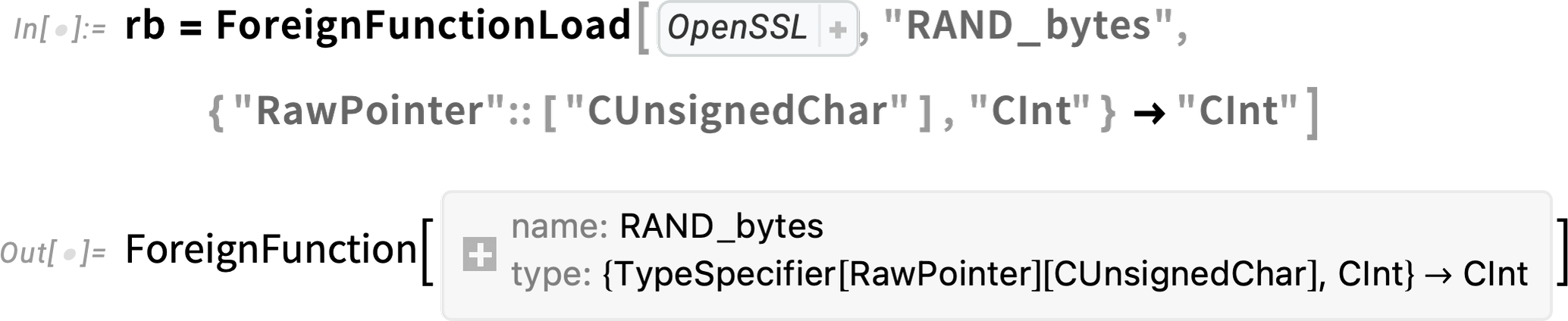
As an example, here’s how one sets up a “foreign function” call to a function RAND_bytes in the OpenSSL library:
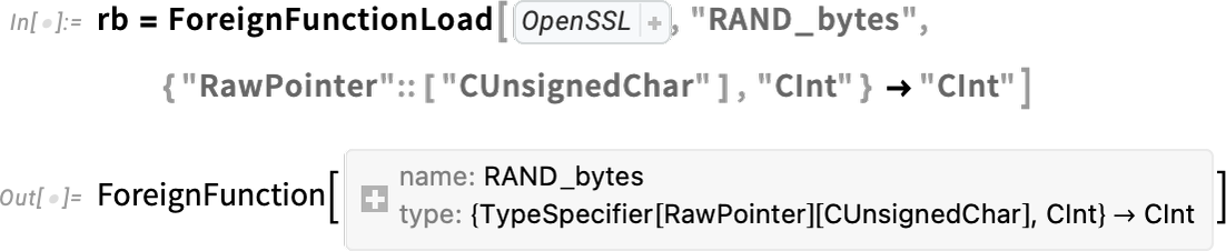
Inside this, we’re using Wolfram Language compiler technology to specify the native C types that will be used in the foreign function. But now we can package this all up into a Wolfram Language function:
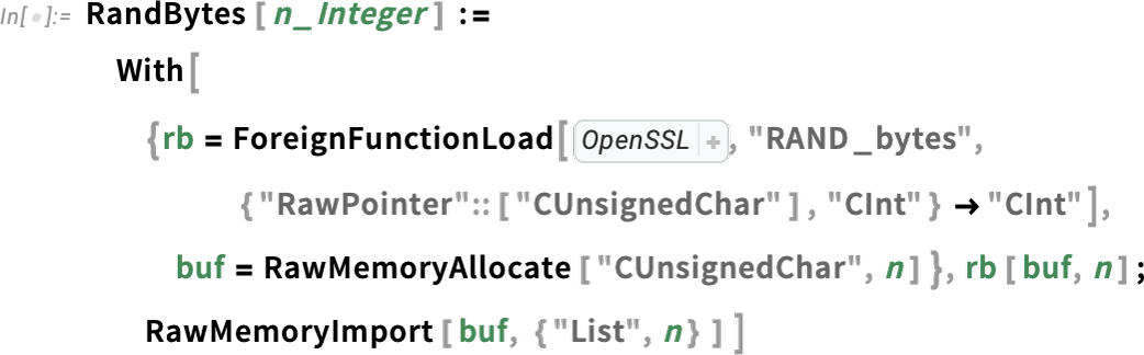
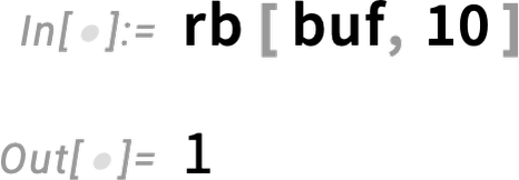
And we can call this function just like any other Wolfram Language function:

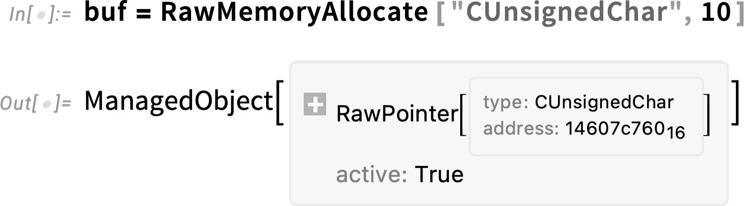
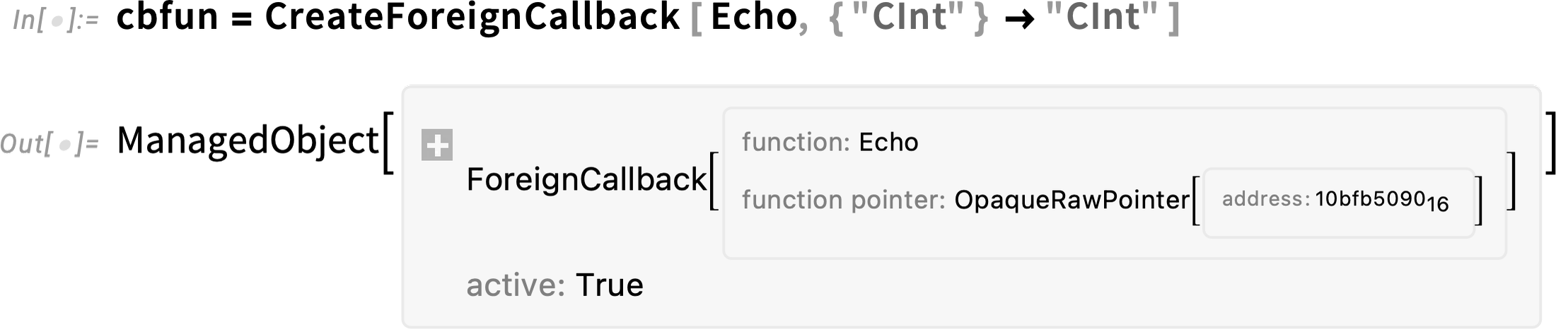
Internally, all sorts of complicated things are going on. For example, we’re allocating a raw memory buffer that’s then getting fed to our C function. But when we do that memory allocation we’re creating a symbolic structure that defines it as a “managed object”:
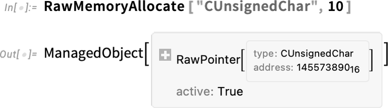
And now when this object is no longer being used, the memory associated with it will be automatically freed.

And, yes, with both Python and C there’s quite a bit of complexity underneath. But the good news is that in Version 14 we’ve basically been able to automate handling it. And the result is that what gets exposed is pure, simple Wolfram Language.

But there’s another big piece to this. Within particular Python or C libraries there are often elaborate definitions of data structures that are specific to that library. And so to use these libraries one has to dive into all the—potentially idiosyncratic—complexities of those definitions. But in the Wolfram Language we have consistent symbolic representations for things, whether they’re images, or dates or types of chemicals. When you first hook up an external library you have to map its data structures to these. But once that’s done, anyone can use what’s been built, and seamlessly integrate with other things they’re doing, perhaps even calling other external code. In effect what’s happening is that one’s leveraging the whole design framework of the Wolfram Language, and applying that even when one’s using underlying implementations that aren’t based on the Wolfram Language.

For Serious Developers

A single line (or less) of Wolfram Language code can do a lot. But one of the remarkable things about the language is that it’s fundamentally scalable: good both for very short programs and very long programs. And since Version 13 there’ve been several advances in handling very long programs. One of them concerns “code editing”.

Standard Wolfram Notebooks work very well for exploratory, expository and many other forms of work. And it’s certainly possible to write large amounts of code in standard notebooks (and, for example, I personally do it). But when one’s doing “software-engineering-style work” it’s both more convenient and more familiar to use what amounts to a pure code editor, largely separate from code execution and exposition. And this is why we have the “package editor”, accessible from File > New > Package/Script. You’re still operating in the notebook environment, with all its sophisticated capabilities. But things have been “skinned” to provide a much more textual “code experience”—both in terms of editing, and in terms of what actually gets saved in .wl files.

Here’s typical example of the package editor in action (in this case applied to our GitLink package):

Package editor

Several things are immediately evident. First, it’s very line oriented. Lines (of code) are numbered, and don’t break except at explicit newlines. There are headings just like in ordinary notebooks, but when the file is saved, they’re stored as comments with a certain stylized structure:

Lines of code

It’s still perfectly possible to run code in the package editor, but the output won’t get saved in the .wl file:

Unsaved output

One thing that’s changed since Version 13 is that the toolbar is much enhanced. And for example there’s now “smart search” that is aware of code structure:

Smart search

You can also ask to go to a line number—and you’ll immediately see whatever lines of code are nearby:

Nearby lines of code

In addition to code editing, another set of features new since Version 13 of importance to serious developers concern automated testing. The main advance is the introduction of a fully symbolic testing framework, in which individual tests are represented as symbolic objects
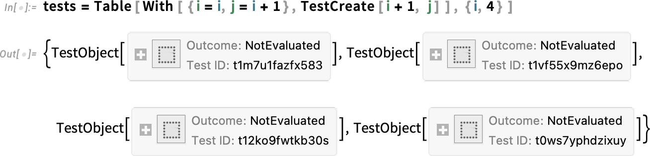
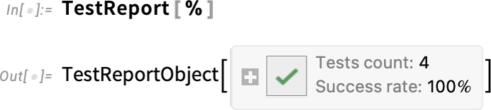
and can be manipulated in symbolic form, then run using functions like TestEvaluate and TestReport:
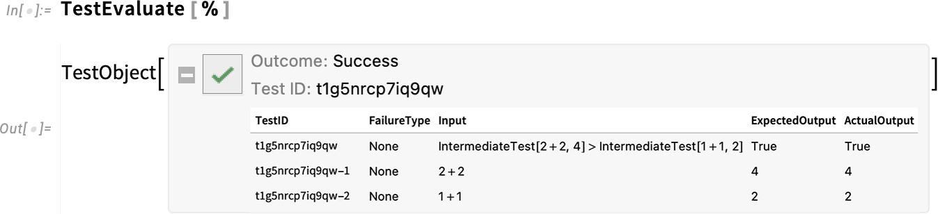
In Version 14.0 there’s another new testing function—IntermediateTest—that lets you insert what amount to checkpoints inside larger tests:

Evaluating this test, we see that the intermediate tests were also run:
Wolfram Function Repository: 2900 Functions & Counting

The Wolfram Function Repository has been a big success. We introduced it in 2019 as a way to make specific, individual contributed functions available in the Wolfram Language. And now there are more than 2900 such functions in the Repository.

The nearly 7000 functions that constitute the Wolfram Language as it is today have been painstakingly developed over the past three and a half decades, always mindful of creating a coherent whole with consistent design principles. And now in a sense the success of the Function Repository is one of the dividends of all that effort. Because it’s the coherence and consistency of the underlying language and its design principles that make it feasible to just add one function at a time, and have it really work. You want to add a function to do some very specific operation that combines images and graphs. Well, there’s a consistent representation of both images and graphs in the Wolfram Language, which you can leverage. And by following the principles of the Wolfram Language—like for the naming of functions—you can create a function that’ll be easy for Wolfram Language users to understand and use.

Using the Wolfram Function Repository is a remarkably seamless process. If you know the function’s name, you can just call it using ResourceFunction; the function will be loaded if it’s needed, and then it’ll just run:

If there’s an update available for the function, it’ll give you a message, but run the old version anyway. The message has a button that lets you load in the update; then you can rerun your input and use the new version. (If you’re writing code where you want to “burn in” a particular version of a function, you can just use the ResourceVersion option of ResourceFunction.)

If you want your code to look more elegant, just evaluate the ResourceFunction object

and use the formatted version:

And, by the way, pressing the + then gives you more information about the function:

Function information

An important feature of functions in the Function Repository is that they all have documentation pages—that are organized pretty much like the pages for built-in functions:

SolarEclipseIcon function page

But how does one create a Function Repository entry? Just go to File > New > Repository Item > Function Repository Item and you’ll get a Definition Notebook:

Definition notebook

We’ve optimized this to be as easy to fill in as possible, minimizing boilerplate and automatically checking for correctness and consistency whenever possible. And the result is that it’s perfectly realistic to create a simple Function Repository item in under an hour—with the main time spent being in the writing of good expository examples.

When you press Submit to Repository your function gets sent to the Wolfram Function Repository review team, whose mandate is to ensure that functions in the repository do what they say they do, work in a way that is consistent with general Wolfram Language design principles, have good names, and are adequately documented. Except for very specialized functions, the goal is to finish reviews within a week (and sometimes considerably sooner)—and to publish functions as soon as they are ready.

There’s a digest of new (and updated) functions in the Function Repository that gets sent out every Friday—and makes for interesting reading (you can subscribe here):

Wolfram Function Repository email

The Wolfram Function Repository is a curated public resource that can be accessed from any Wolfram Language system (and, by the way, the source code for every function is available—just press the Source Notebook button). But there’s another important use case for the infrastructure of the Function Repository: privately deployed “resource functions”.

It all works through the Wolfram Cloud. You use the exact same Definition Notebook, but now instead of submitting to the public Wolfram Function Repository, you just deploy your function to the Wolfram Cloud. You can make it private so that only you, or some specific group, can access it. Or you can make it public, so anyone who knows its URL can immediately access and use it in their Wolfram Language system.

This turns out to be a tremendously useful mechanism, both for group projects, and for creating published material. In a sense it’s a very lightweight but robust way to distribute code—packaged into functions that can immediately be used. (By the way, to find the functions you’ve published from your Wolfram Cloud account, just go to the DeployedResources folder in the cloud file browser.)

(For organizations that want to manage their own function repository, it’s worth mentioning that the whole Wolfram Function Repository mechanism—including the infrastructure for doing reviews, etc.—is also available in a private form through the Wolfram Enterprise Private Cloud.)

So what’s in the public Wolfram Function Repository? There are a lot of “specialty functions” intended for specific “niche” purposes—but very useful if they’re what you want:

There are functions that add various kinds of visualizations:

Some functions set up user interfaces:

Some functions link to external services:

Some functions provide simple utilities:

There are also functions that are being explored for potential inclusion in the core system:

There are also lots of “leading-edge” functions, added as part of research or exploratory development. And for example in pieces I write (including this one), I make a point of having all pictures and other output be backed by “click-to-copy” code that reproduces them—and this code quite often contains functions either from the public Wolfram Function Repository or from (publicly accessible) private deployments.

The Paclet Repository Arrives

Paclets are a technology we’ve used for more than a decade and a half to distribute updated functionality to Wolfram Language systems in the field. In Version 13 we began the process of providing tools for anyone to create paclets. And since Version 13 we’ve introduced the Wolfram Language Paclet Repository as a centralized repository for paclets:

Wolfram Paclet Repository

What is a paclet? It’s a collection of Wolfram Language functionality—including function definitions, documentation, external libraries, stylesheets, palettes and more—that can be distributed as a unit, and immediately deployed in any Wolfram Language system.

The Paclet Repository is a centralized place where anyone can publish paclets for public distribution. So how does this relate to the Wolfram Function Repository? They are interestingly complementary—with different optimization and different setups. The Function Repository is more lightweight, the Paclet Repository more flexible. The Function Repository is for making available individual new functions, that independently fit into the whole existing structure of the Wolfram Language. The Paclet Repository is for making available larger-scale pieces of functionality, that can define a whole framework and environment of their own.

The Function Repository is also fully curated, with every function being reviewed by our team before it is posted. The Paclet Repository is an immediate-deployment system, without pre-publication review. In the Function Repository every function is specified just by its name—and our review team is responsible for ensuring that names are well chosen and have no conflicts. In the Paclet Repository, every contributor gets their own namespace, and all their functions and other material live inside that namespace. So, for example, I contributed the function RandomHypergraph to the Function Repository, which can be accessed just as ResourceFunction["RandomHypergraph"]. But if I had put this function in a paclet in the Paclet Repository, it would have to be accessed as something like PacletSymbol["StephenWolfram/Hypergraphs", "RandomHypergraph"].

PacletSymbol, by the way, is a convenient way of “deep accessing” individual functions inside a paclet. PacletSymbol temporarily installs (and loads) a paclet so that you can access a particular symbol in it. But more often one wants to permanently install a paclet (using PacletInstall), then explicitly load its contents (using Needs) whenever one wants to have its symbols available. (All the various ancillary elements, like documentation, stylesheets, etc. in a paclet get set up when it is installed.)

What does a paclet look like in the Paclet Repository? Every paclet has a home page that typically includes an overall summary, a guide to the functions in the paclet, and some overall examples of the paclet:

ProteinVisualization page

Individual functions typically have their own documentation pages:

AmidePlanePlot page

Just like in the main Wolfram Language documentation, there can be a whole hierarchy of guide pages, and there can be things like tutorials.

Notice that in examples in paclet documentation, one often sees constructs like . These represent symbols in the paclet, presented in forms like PacletSymbol["WolframChemistry/ProteinVisualization", "AmidePlanePlot"] that allow these symbols to be accessed in a “standalone” way. If you directly evaluate such a form, by the way, it’ll force (temporary) installation of the paclet, then return the actual, raw symbol that appears in the paclet:

So how does one create a paclet suitable for submission to the Paclet Repository? You can do it purely programmatically, or you can start from File > New > Repository Item > Paclet Repository Item, which launches what amounts to a whole paclet creation IDE. The first step is to specify where you want to assemble your paclet. You give some basic information

Submit paclet information

then a Paclet Resource Definition Notebook is created, from which you can give function definitions, set up documentation pages, specify what you want your paclet’s home page to be like, etc.:

Paclet Resource Definition Notebook

There are lots of sophisticated tools that let you create full-featured paclets with the same kind of breadth and depth of capabilities that you find in the Wolfram Language itself. For example, Documentation Tools lets you construct full-featured documentation pages (function pages, guide pages, tutorials, …):

Documentation Tools

Once you’ve assembled a paclet, you can check it, build it, deploy it privately—or submit it to the Paclet Repository. And once you submit it, it will automatically get set up on the Paclet Repository servers, and within just a few minutes the pages you’ve created describing your paclet will show up on the Paclet Repository website.

So what’s in the Paclet Repository so far? There’s a lot of good and very serious stuff, contributed both by teams at our company and by members of the broader Wolfram Language community. In fact, many of the 134 paclets now in the Paclet Repository have enough in them that there’s a whole piece like this that one could write about them.

One category of things you’ll find in the Paclet Repository are snapshots of our ongoing internal development projects—many of which will eventually become built-in parts of the Wolfram Language. A good example of this is our LLM and Chat Notebook functionality, whose rapid development and deployment over the past year was made possible by the use of the Paclet Repository. Another example, representing ongoing work from our chemistry team (AKA WolframChemistry in the Paclet Repository) is the ChemistryFunctions paclet, which contains functions like:

And, yes, this is interactive:

Or, also from WolframChemistry:

Another “development snapshot” is DiffTools—a paclet for making and viewing diffs between strings, cells, notebooks, etc.:

A major paclet is QuantumFramework—which provides the functionality for our Wolfram Quantum Framework

Wolfram Quantum Framework

and delivers broad support for quantum computing (with at least a few connections to multiway systems and our Physics Project):

Talking of our Physics Project, there are over 200 functions supporting it that are in the Wolfram Function Repository. But there are also paclets, like WolframInstitute/Hypergraph:

An example of an externally contributed package is Automata—with more than 250 functions for doing computations related to finite automata:

Another contributed paclet is FunctionalParsers, which goes from a symbolic parser specification to an actual parser, here being used in a reverse mode to generate random “sentences”:

Phi4Tools is a more specialized paclet, for working with Feynman diagrams in field theory:

And, as another example, here’s MaXrd, for crystallography and x-ray scattering:

As just one more example, there’s the Organizer paclet—a utility paclet for making and manipulating organizer notebooks. But unlike the other paclets we’ve seen here, it doesn’t expose any Wolfram Language functions; instead, when you install it, it puts a palette in your Palettes list:

Organizer

Coming Attractions

As of today, Version 14 is finished, and out in the world. So what’s next? We have lots of projects underway—some already with years of development behind them. Some extend and strengthen what’s already in the Wolfram Language; some take it in new directions.

One major focus is broadening and streamlining the deployment of the language: unifying the way it’s delivered and installed on computers, packaging it so it can be efficiently integrated into other standalone applications, etc.

Another major focus is expanding the handling of very large amounts of data by the Wolfram Language—and seamlessly integrating out-of-core and lazy processing.

Then of course there’s algorithmic development. Some is “classical”, directly building on the towers of functionality we’ve developed over the decades. Some is more “AI based”. We’ve been creating heuristic algorithms and meta-algorithms ever since Version 1.0—increasingly using methods from machine learning. How far will neural net methods go? We don’t know yet. We’re routinely using them in things like algorithm selection. But to what extent can they help in the heart of algorithms?

I’m reminded of something we did back in 1987 in developing Version 1.0. There was a long tradition in numerical analysis of painstakingly deriving series approximations for particular cases of mathematical functions. But we wanted to be able to compute hundreds of different functions to arbitrary precision for any complex values of their arguments. So how did we do it? We generalized from series to rational approximations—and then, in a very “machine-learning-esque” way—we spent months of CPU time systematically optimizing these approximations. Well, we’ve been trying to do the same kind of thing again—though now over more ambitious domains—and now using not rational functions but large neural nets as our basis.

We’ve also been exploring using neural nets to “control” precise algorithms, in effect making heuristic choices which either guide or can be validated by the precise algorithms. So far, none of what we’ve produced has outperformed our existing methods, but it seems plausible that fairly soon it will.

We’re doing a lot with various aspects of metaprogramming. There’s the project of
getting LLMs to help in the construction of Wolfram Language code—and in giving comments on it, and in analyzing what went wrong if the code didn’t do what one expected. Then there’s code annotation—where LLMs may help in doing things like predicting the most likely type for something. And there’s code compilation. We’ve been working for many years on a full-scale compiler for the Wolfram Language, and in every version what we have becomes progressively more capable. We’ve been doing some level of automatic compilation in particular cases (particularly ones involving numerical computation) for more than 30 years. And eventually full-scale automatic compilation will be possible for everything. But as of now some of the biggest payoffs from our compiler technology have been for our internal development, where we can now get optimal down-to-the-metal performance simply by compiled (albeit carefully written) Wolfram Language code.

One of the big lessons of the surprising success of LLMs is that there’s potentially more structure in meaningful human language than we thought. I’ve long been interested in creating what I’ve called a “symbolic discourse language” that gives a computational representation of everyday discourse. The LLMs haven’t explicitly done that. But they encourage the idea that it should be possible, and they also provide practical help in doing it. And whether the goal is to be able to represent narrative text, or contracts, or textual specifications, it’s a matter of extending the computational language we’ve built to encompass more kinds of concepts and structures.

There are typically several kinds of drivers for our continued development efforts. Sometimes it’s a question of continuing to build a tower of capabilities in some known direction (like, for example, solving PDEs). Sometimes the tower we’ve built suddenly lets us see new possibilities. Sometimes when we actually use what we’ve built we realize there’s an obvious way to polish or extend it—or to “double down” on something that we can now see is valuable. And then there are cases where things happening in the technology world suddenly open up new possibilities—like LLMs have recently done, and perhaps XR will eventually do. And finally there are cases where new science-related insights suggest new directions.

I had assumed that our Physics Project would at best have practical applications only centuries hence. But in fact it’s become clear that the correspondence it’s defined between physics and computation gives us quite immediate new ways to think about aspects of practical computation. And indeed we’re now actively exploring how to use this to define a new level of parallel and distributed computation in the Wolfram Language, as well as to represent symbolically not only the results of computations but also the ongoing process of computation.

One might think that after nearly four decades of intense development there wouldn’t be anything left to do in developing the Wolfram Language. But in fact at every level we reach, there’s ever more that becomes possible, and ever more that can we see might be possible. And indeed this moment is a particularly fertile one, with an unprecedentedly broad waterfront of possibilities. Version 14 is an important and satisfying waypoint. But there are wonderful things ahead—as we continue our long-term mission to make the computational paradigm achieve its potential, and to build our computational language to help that happen.

🔲 ☆

LLM Tech and a Lot More: Version 13.3 of Wolfram Language and Mathematica

LLM Tech and a Lot More: Version 13.3 of Wolfram Language and Mathematica

The Leading Edge of 2023 Technology … and Beyond

Today we’re launching Version 13.3 of Wolfram Language and Mathematica—both available immediately on desktop and cloud. It’s only been 196 days since we released Version 13.2, but there’s a lot that’s new, not least a whole subsystem around LLMs.

Last Friday (June 23) we celebrated 35 years since Version 1.0 of Mathematica (and what’s now Wolfram Language). And to me it’s incredible how far we’ve come in these 35 years—yet how consistent we’ve been in our mission and goals, and how well we’ve been able to just keep building on the foundations we created all those years ago.

And when it comes to what’s now Wolfram Language, there’s a wonderful timelessness to it. We’ve worked very hard to make its design as clean and coherent as possible—and to make it a timeless way to elegantly represent computation and everything that can be described through it.

Last Friday I fired up Version 1 on an old Mac SE/30 computer (with 2.5 megabytes of memory), and it was a thrill see functions like Plot and NestList work just as they would today—albeit a lot slower. And it was wonderful to be able to take (on a floppy disk) the notebook I created with Version 1 and have it immediately come to life on a modern computer.

But even as we’ve maintained compatibility over all these years, the scope of our system has grown out of all recognition—with everything in Version 1 now occupying but a small sliver of the whole range of functionality of the modern Wolfram Language:

Versions 1.0 and 13.3 of Wolfram Language compared

So much about Mathematica was ahead of its time in 1988, and perhaps even more about Mathematica and the Wolfram Language is ahead of its time today, 35 years later. From the whole idea of symbolic programming, to the concept of notebooks, the universal applicability of symbolic expressions, the notion of computational knowledge, and concepts like instant APIs and so much more, we’ve been energetically continuing to push the frontier over all these years.

Our long-term objective has been to build a full-scale computational language that can represent everything computationally, in a way that’s effective for both computers and humans. And now—in 2023—there’s a new significance to this. Because with the advent of LLMs our language has become a unique bridge between humans, AIs and computation.

The attributes that make Wolfram Language easy for humans to write, yet rich in expressive power, also make it ideal for LLMs to write. And—unlike traditional programming languages— Wolfram Language is intended not only for humans to write, but also to read and think in. So it becomes the medium through which humans can confirm or correct what LLMs do, to deliver computational language code that can be confidently assembled into a larger system.

The Wolfram Language wasn’t originally designed with the recent success of LLMs in mind. But I think it’s a tribute to the strength of its design that it now fits so well with LLMs—with so much synergy. The Wolfram Language is important to LLMs—in providing a way to access computation and computational knowledge from within the LLM. But LLMs are also important to Wolfram Language—in providing a rich linguistic interface to the language.

We’ve always built—and deployed—Wolfram Language so it can be accessible to as many people as possible. But the advent of LLMs—and our new Chat Notebooks—opens up Wolfram Language to vastly more people. Wolfram|Alpha lets anyone use natural language—without prior knowledge—to get questions answered. Now with LLMs it’s possible to use natural language to start defining potential elaborate computations.

As soon as you’ve formulated your thoughts in computational terms, you can immediately “explain them to an LLM”, and have it produce precise Wolfram Language code. Often when you look at that code you’ll realize you didn’t explain yourself quite right, and either the LLM or you can tighten up your code. But anyone—without any prior knowledge—can now get started producing serious Wolfram Language code. And that’s very important in seeing Wolfram Language realize its potential to drive “computational X” for the widest possible range of fields X.

But while LLMs are “the biggest single story” in Version 13.3, there’s a lot else in Version 13.3 too—delivering the latest from our long-term research and development pipeline. So, yes, in Version 13.3 there’s new functionality not only in LLMs but also in many “classic” areas—as well as in new areas having nothing to do with LLMs.

Across the 35 years since Version 1 we’ve been able to continue accelerating our research and development process, year by year building on the functionality and automation we’ve created. And we’ve also continually honed our actual process of research and development—for the past 5 years sharing our design meetings on open livestreams.

Version 13.3 is—from its name—an “incremental release”. But—particularly with its new LLM functionality—it continues our tradition of delivering a long list of important advances and updates, even in incremental releases.

LLM Tech Comes to Wolfram Language

LLMs make possible many important new things in the Wolfram Language. And since I’ve been discussing these in a series of recent posts, I’ll just give only a fairly short summary here. More details are in the other posts, both ones that have appeared, and ones that will appear soon.

To ensure you have the latest Chat Notebook functionality installed and available, use:

PacletInstall["Wolfram/Chatbook" "1.0.0", UpdatePacletSites True].

The most immediately visible LLM tech in Version 13.3 is Chat Notebooks. Go to File > New > Chat-Enabled Notebook and you’ll get a Chat Notebook that supports “chat cells” that let you “talk to” an LLM. Press ' (quote) to get a new chat cell:

Plot two sine curves

You might not like some details of what got done (do you really want those boldface labels?) but I consider this pretty impressive. And it’s a great example of using an LLM as a “linguistic interface” with common sense, that can generate precise computational language, which can then be run to get a result.

This is all very new technology, so we don’t yet know what patterns of usage will work best. But I think it’s going to go like this. First, you have to think computationally about whatever you’re trying to do. Then you tell it to the LLM, and it’ll produce Wolfram Language code that represents what it thinks you want to do. You might just run that code (or the Chat Notebook will do it for you), and see if it produces what you want. Or you might read the code, and see if it’s what you want. But either way, you’ll be using computational language—Wolfram Language—as the medium to formalize and express what you’re trying to do.

When you’re doing something you’re familiar with, it’ll almost always be faster and better to think directly in Wolfram Language, and just enter the computational language code you want. But if you’re exploring something new, or just getting started on something, the LLM is likely to be a really valuable way to “get you to first code”, and to start the process of crispening up what you want in computational terms.

If the LLM doesn’t do exactly what you want, then you can tell it what it did wrong, and it’ll try to correct it—though sometimes you can end up doing a lot of explaining and having quite a long dialog (and, yes, it’s often vastly easier just to type Wolfram Language code yourself):

Draw red and green semicircles

Redraw red and green semicircles

Sometimes the LLM will notice for itself that something went wrong, and try changing its code, and rerunning it:

Make table of primes

And even if it didn’t write a piece of code itself, it’s pretty good at piping up to explain what’s going on when an error is generated:

Error report

And actually it’s got a big advantage here, because “under the hood” it can look at lots of details (like stack trace, error documentation, etc.) that humans usually don’t bother with.

To support all this interaction with LLMs, there’s all kinds of new structure in the Wolfram Language. In Chat Notebooks there are chat cells, and there are chatblocks (indicated by gray bars, and generating with ~) that delimit the range of chat cells that will be fed to the LLM when you press shiftenter on a new chat cell. And, by the way, the whole mechanism of cells, cell groups, etc. that we invented 36 years ago now turns out to be extremely powerful as a foundation for Chat Notebooks.

One can think of the LLM as a kind of “alternate evaluator” in the notebook. And there are various ways to set up and control it. The most immediate is in the menu associated with every chat cell and every chatblock (and also available in the notebook toolbar):

Chat cell and chatblock menu

The first items here let you define the “persona” for the LLM. Is it going to act as a Code Assistant that writes code and comments on it? Or is it just going to be a Code Writer, that writes code without being wordy about it? Then there are some “fun” personas—like Wolfie and Birdnardo—that respond “with an attitude”. The Advanced Settings let you do things like set the underlying LLM model you want to use—and also what tools (like Wolfram Language code evaluation) you want to connect to it.

Ultimately personas are mostly just special prompts for the LLM (together, sometimes with tools, etc.) And one of the new things we’ve recently launched to support LLMs is the Wolfram Prompt Repository:

Wolfram Prompt Repository

The Prompt Repository contains several kinds of prompts. The first are personas, which are used to “style” and otherwise inform chat interactions. But then there are two other types of prompts: function prompts, and modifier prompts.

Function prompts are for getting the LLM to do something specific, like summarize a piece of text, or suggest a joke (it’s not terribly good at that). Modifier prompts are for determining how the LLM should modify its output, for example translating into a different human language, or keeping it to a certain length.

You can pull in function prompts from the repository into a Chat Notebook by using !, and modifier prompts using #. There’s also a ^ notation for saying that you want the “input” to the function prompt to be the cell above:

ScientificJargonize

This is how you can access LLM functionality from within a Chat Notebook. But there’s also a whole symbolic programmatic way to access LLMs that we’ve added to the Wolfram Language. Central to this is LLMFunction, which acts very much like a Wolfram Language pure function, except that it gets “evaluated” not by the Wolfram Language kernel, but by an LLM:

You can access a function prompt from the Prompt Repository using LLMResourceFunction:

There’s also a symbolic representation for chats. Here’s an empty chat:

And here now we “say something”, and the LLM responds:

There’s lots of depth to both Chat Notebooks and LLM functionsas I’ve described elsewhere. There’s LLMExampleFunction for getting an LLM to follow examples you give. There’s LLMTool for giving an LLM a way to call functions in the Wolfram Language as “tools”. And there’s LLMSynthesize which provides raw access to the LLM as its text completion and other capabilities. (And controlling all of this is $LLMEvaluator which defines the default LLM configuration to use, as specified by an LLMConfiguration object.)

I consider it rather impressive that we’ve been able to get to the level of support for LLMs that we have in Version 13.3 in less than six months (along with building things like the Wolfram Plugin for ChatGPT, and the Wolfram ChatGPT Plugin Kit). But there’s going to be more to come, with LLM functionality increasingly integrated into Wolfram Language and Notebooks, and, yes, Wolfram Language functionality increasingly integrated as a tool into LLMs.

Line, Surface and Contour Integration

“Find the integral of the function ___” is a typical core thing one wants to do in calculus. And in Mathematica and the Wolfram Language that’s achieved with Integrate. But particularly in applications of calculus, it’s common to want to ask slightly more elaborate questions, like “What’s the integral of ___ over the region ___?”, or “What’s the integral of ___ along the line ___?”

Almost a decade ago (in Version 10) we introduced a way to specify integration over regions—just by giving the region “geometrically” as the domain of the integral:

It had always been possible to write out such an integral in “standard Integrate” form

but the region specification is much more convenient—as well as being much more efficient to process.

Finding an integral along a line is also something that can ultimately be done in “standard Integrate” form. And if you have an explicit (parametric) formula for the line this is typically fairly straightforward. But if the line is specified in a geometrical way then there’s real work to do to even set up the problem in “standard Integrate” form. So in Version 13.3 we’re introducing the function LineIntegrate to automate this.

LineIntegrate can deal with integrating both scalar and vector functions over lines. Here’s an example where the line is just a straight line:

But LineIntegrate also works for lines that aren’t straight, like this parametrically specified one:

To compute the integral also requires finding the tangent vector at every point on the curve—but LineIntegrate automatically does that:

Line integrals are common in applications of calculus to physics. But perhaps even more common are surface integrals, representing for example total flux through a surface. And in Version 13.3 we’re introducing SurfaceIntegrate. Here’s a fairly straightforward integral of flux that goes radially outward through a sphere:

Here’s a more complicated case:

And here’s what the actual vector field looks like on the surface of the dodecahedron:

LineIntegrate and SurfaceIntegrate deal with integrating scalar and vector functions in Euclidean space. But in Version 13.3 we’re also handling another kind of integration: contour integration in the complex plane.

We can start with a classic contour integral—illustrating Cauchy’s theorem:

Here’s a slightly more elaborate complex function

and here’s its integral around a circular contour:

Needless to say, this still gives the same result, since the new contour still encloses the same poles:

More impressively, here’s the result for an arbitrary radius of contour:

And here’s a plot of the (imaginary part of the) result:

Contours can be of any shape:

The result for the contour integral depends on whether the pole is inside the “Pac-Man”:

Another Milestone for Special Functions

One can think of special functions as a way of “modularizing” mathematical results. It’s often a challenge to know that something can be expressed in terms of special functions. But once one’s done this, one can immediately apply the independent knowledge that exists about the special functions.

Even in Version 1.0 we already supported many special functions. And over the years we’ve added support for many more—to the point where we now cover everything that might reasonably be considered a “classical” special function. But in recent years we’ve also been tackling more general special functions. They’re mathematically more complex, but each one we successfully cover makes a new collection of problems accessible to exact solution and reliable numerical and symbolic computation.

Most of the “classic” special functions—like Bessel functions, Legendre functions, elliptic integrals, etc.—are in the end univariate hypergeometric functions. But one important frontier in “general special functions” are those corresponding to bivariate hypergeometric functions. And already in Version 4.0 (1999) we introduced one example of such as a function: AppellF1. And, yes, it’s taken a while, but now in Version 13.3 we’ve finally finished doing the math and creating the algorithms to introduce AppellF2, AppellF3 and AppellF4.

On the face of it, it’s just another function—with lots of arguments—whose value we can find to any precision:

Occasionally it has a closed form:

But despite its mathematical sophistication, plots of it tend to look fairly uninspiring:

Series expansions begin to show a little more:

And ultimately this is a function that solves a pair of PDEs that can be seen as a generalization to two variables of the univariate hypergeometric ODE. So what other generalizations are possible? Paul Appell spent many years around the turn of the twentieth century looking—and came up with just four, which as of Version 13.3 now all appear in the Wolfram Language, as AppellF1, AppellF2, AppellF3 and AppellF4.

To make special functions useful in the Wolfram Language they need to be “knitted” into other capabilities of the language—from numerical evaluation to series expansion, calculus, equation solving, and integral transforms. And in Version 13.3 we’ve passed another special function milestone, around integral transforms.

When I started using special functions in the 1970s the main source of information about them tended to be a small number of handbooks that had been assembled through decades of work. When we began to build Mathematica and what’s now the Wolfram Language, one of our goals was to subsume the information in such handbooks. And over the years that’s exactly what we’ve achieved—for integrals, sums, differential equations, etc. But one of the holdouts has been integral transforms for special functions. And, yes, we’ve covered a great many of these. But there are exotic examples that can often only “coincidentally” be done in closed form—and that in the past have only been found in books of tables.

But now in Version 13.3 we can do cases like:

And in fact we believe that in Version 13.3 we’ve reached the edge of what’s ever been figured out about Laplace transforms for special functions. The most extensive handbook—finally published in 1973—runs to about 400 pages. A few years ago we could do about 55% of the forward Laplace transforms in the book, and 31% of the inverse ones. But now in Version 13.3 we can do 100% of the ones that we can verify as correct (and, yes, there are definitely some mistakes in the book). It’s the end of a long journey, and a satisfying achievement in the quest to make as much mathematical knowledge as possible automatically computable.

Finite Fields!

Ever since Version 1.0 we’ve been able to do things like factoring polynomials modulo primes. And many packages have been developed that handle specific aspects of finite fields. But in Version 13.3 we now have complete, consistent coverage of all finite fields—and operations with them.

Here’s our symbolic representation of the field of integers modulo 5 (AKA ℤ5 or GF(5)):

And here are symbolic representations of the elements of this field—which in this particular case can be rather trivially identified with ordinary integers mod 5:

Arithmetic immediately works on these symbolic elements:

But where things get a bit trickier is when we’re dealing with prime-power fields. We represent the field GF(23) symbolically as:

But now the elements of this field no longer have a direct correspondence with ordinary integers. We can still assign “indices” to them, though (with elements 0 and 1 being the additive and multiplicative identities). So here’s an example of an operation in this field:

But what actually is this result? Well, it’s an element of the finite field—with index 4—represented internally in the form:

The little box opens out to show the symbolic FiniteField construct:

FormField construct

And we can extract properties of the element, like its index:

So here, for example, are the complete addition and multiplication tables for this field:

For the field GF(72) these look a little more complicated:

There are various number-theoretic-like functions that one can compute for elements of finite fields. Here’s an element of GF(510):

The multiplicative order of this (i.e. power of it that gives 1) is quite large:

Here’s its minimal polynomial:

But where finite fields really begin to come into their own is when one looks at polynomials over them. Here, for example, is factoring over GF(32):

Expanding this gives a finite-field-style representation of the original polynomial:

Here’s the result of expanding a power of a polynomial over GF(32):

More, Stronger Computational Geometry

We originally introduced computational geometry in a serious way into the Wolfram Language a decade ago. And ever since then we’ve been building more and more capabilities in computational geometry.

We’ve had RegionDistance for computing the distance from a point to a region for a decade. In Version 13.3 we’ve now extended RegionDistance so it can also compute the shortest distance between two regions:

We’ve also introduced RegionFarthestDistance which computes the furthest distance between any two points in two given regions:

Another new function in Version 13.3 is RegionHausdorffDistance which computes the largest of all shortest distances between points in two regions; in this case it gives a closed form:

Another pair of new functions in Version 13.3 are InscribedBall and CircumscribedBall—which give (n-dimensional) spheres that, respectively, just fit inside and outside regions you give:

In the past several versions, we’ve added functionality that combines geo computation with computational geometry. Version 13.3 has the beginning of another initiative—introducing abstract spherical geometry:

This works for spheres in any number of dimensions:

In addition to adding functionality, Version 13.3 also brings significant speed enhancements (often 10x or more) to some core operations in 2D computational geometry—making things like computing this fast even though it involves complicated regions:

Visualizations Begin to Come Alive

A great long-term strength of the Wolfram Language has been its ability to produce insightful visualizations in a highly automated way. In Version 13.3 we’re taking this further, by adding automatic “live highlighting”. Here’s a simple example, just using the function Plot. Instead of just producing static curves, Plot now automatically generates a visualization with interactive highlighting:

The same thing works for ListPlot:

The highlighting can, for example, show dates too:

There are many choices for how the highlighting should be done. The simplest thing is just to specify a style in which to highlight whole curves:

But there are many other built-in highlighting specifications. Here, for example, is "XSlice":

In the end, though, highlighting is built up from a whole collection of components—like "NearestPoint", "Crosshairs", "XDropline", etc.—that you can assemble and style for yourself:

The option PlotHighlighting defines global highlighting in a plot. But by using the Highlighted “wrapper” you can specify that only a particular element in the plot should be highlighted:

For interactive and exploratory purposes, the kind of automatic highlighting we’ve just been showing is very convenient. But if you’re making a static presentation, you’ll need to “burn in” particular pieces of highlighting—which you can do with Placed:

In indicating elements in a graphic there are different effects one can use. In Version 13.1 we introduced DropShadowing[]. In Version 13.3 we’re introducing Haloing:

Haloing can also be combined with interactive highlighting:

By the way, there are lots of nice effects you can get with Haloing in graphics. Here’s a geo example—including some parameters for the “orientation” and “thickness” of the haloing:

Publishing to Augmented + Virtual Reality

Throughout the history of the Wolfram Language 3D visualization has been an important capability. And we’re always looking for ways to share and communicate 3D geometry. Already back in the early 1990s we had experimental implementations of VR. But at the time there wasn’t anything like the kind of infrastructure for VR that would be needed to make this broadly useful. In the mid-2010s we then introduced VR functionality based on Unity—that provides powerful capabilities within the Unity ecosystem, but is not accessible outside.

Today, however, it seems there are finally broad standards emerging for AR and VR. And so in Version 13.3 we’re able to begin delivering what we hope will provide widely accessible AR and VR deployment from the Wolfram Language.

At a underlying level what we’re doing is to support the USD and GLTF geometry representation formats. But we’re also building a higher-level interface that allows anyone to “publish” 3D geometry for AR and VR.

Given a piece of geometry (which for now can’t involve too many polygons), all you do is apply ARPublish:

The result is a cloud object that has a certain underlying UUID, but is displayed in a notebook as a QR code. Now all you do is look at this QR code with your phone (or tablet, etc.) camera, and press the URL it extracts.

The result will be that the geometry you published with ARPublish now appears in AR on your phone:

Augmented reality triptych

Move your phone and you’ll see that your geometry has been realistically placed into the scene. You can also go to a VR “object” mode in which you can manipulate the geometry on your phone.

“Under the hood” there are some slightly elaborate things going on—particularly in providing the appropriate data to different kinds of phones. But the result is a first step in the process of easily being able to get AR and VR output from the Wolfram Language—deployed in whatever devices support AR and VR.

Getting the Details Right: The Continuing Story

In every version of Wolfram Language we add all sorts of fundamentally new capabilities. But we also work to fill in details of existing capabilities, continually pushing to make them as general, consistent and accurate as possible. In Version 13.3 there are many details that have been “made right”, in many different areas.

Here’s one example: the comparison (and sorting) of Around objects. Here are 10 random “numbers with uncertainty”:

These sort by their central value:

But if we look at these, many of their uncertainty regions overlap:

So when should we consider a particular number-with-uncertainty “greater than” another? In Version 13.3 we carefully take into account uncertainty when making comparisons. So, for example, this gives True:

But when there’s too big an uncertainty in the values, we no longer consider the ordering “certain enough”:

Here’s another example of consistency: the applicability of Duration. We introduced Duration to apply to explicit time constructs, things like Audio objects, etc. But in Version 13.3 it also applies to entities for which there’s a reasonable way to define a “duration”:

Dates (and times) are complicated things—and we’ve put a lot of effort into handling them correctly and consistently in the Wolfram Language. One concept that we introduced a few years ago is date granularity: the (subtle) analog of numerical precision for dates. But at first only some date functions supported granularity; now in Version 13.3 all date functions include a DateGranularity option—so that granularity can consistently be tracked through all date-related operations:

Also in dates, something that’s been added, particularly for astronomy, is the ability to deal with “years” specified by real numbers:

And one consequence of this is that it becomes easier to make a plot of something like astronomical distance as a function of time:

Also in astronomy, we’ve been steadily extending our capabilities to consistently fill in computations for more situations. In Version 13.3, for example, we can now compute sunrise, etc. not just from points on Earth, but from points anywhere in the solar system:

By the way, we’ve also made the computation of sunrise more precise. So now if you ask for the position of the Sun right at sunrise you’ll get a result like this:

How come the altitude of the Sun is not zero at sunrise? That’s because the disk of the Sun is of nonzero size, and “sunrise” is defined to be when any part of the Sun pokes over the horizon.

Even Easier to Type: Affordances for Wolfram Language Input

Back in 1988 when what’s now Wolfram Language first existed, the only way to type it was like ordinary text. But gradually we’ve introduced more and more “affordances” to make it easier and faster to type correct Wolfram Language input. In 1996, with Version 3, we introduced automatic spacing (and spanning) for operators, as well as brackets that flashed when they matched—and things like -> being automatically replaced by . Then in 2007, with Version 6, we introduced—with some trepidation at first—syntax coloring. We’d had a way to request autocompletion of a symbol name all the way back to the beginning, but it’d never been good or efficient enough for us to make it happen all the time as you type. But in 2012, for Version 9, we created a much more elaborate autocomplete system—that was useful and efficient enough that we turned it on for all notebook input. A key feature of this autocomplete system was its context-sensitive knowledge of the Wolfram Language, and how and where different symbols and strings typically appear. Over the past decade, we’ve gradually refined this system to the point where I, for one, deeply rely on it.

In recent versions, we’ve made other “typability” improvements. For example, in Version 12.3, we generalized the -> to transformation to a whole collection of “auto operator renderings”. Then in Version 13.0 we introduced “automatching” of brackets, in which, for example, if you enter [ at the end of what you’re typing, you’ll automatically get a matching ].

Making “typing affordances” work smoothly is a painstaking and tricky business. But in every recent version we’ve steadily been adding more features that—in very “natural” ways—make it easier and faster to type Wolfram Language input.

In Version 13.3 one major change is an enhancement to autocompletion. Instead of just showing pure completions in which characters are appended to what’s already been typed, the autocompletion menu now includes “fuzzy completions” that fill in intermediate characters, change capitalization, etc.

So, for example, if you type “lp” you now get ListPlot as a completion (the little underlines indicate where the letters you actually type appear):

ListPlot autocompletion menu

From a design point of view one thing that’s important about this is that it further removes the “short name” premium—and weights things even further on the side of wanting names that explain themselves when they’re read, rather than that are easy to type in an unassisted way. With the Wolfram Function Repository it’s become increasingly common to want to type ResourceFunction. And we’d been thinking that perhaps we should have a special, short notation for that. But with the new autocompletion, one can operationally just press three keys—rfenterto get to ResourceFunction:

ResourceFunction autocompletion menu

When one designs something and gets the design right, people usually don’t notice; things just “work as they expect”. But when there’s a design error, that’s when people notice—and are frustrated by—the design. But then there’s another case: a situation where, for example, there are two things that could happen, and sometimes one wants one, and sometimes the other. In doing the design, one has to pick a particular branch. And when this happens to be the branch people want, they don’t notice, and they’re happy. But if they want the other branch, it can be confusing and frustrating.

In the design of the Wolfram Language one of the things that has to be chosen is the precedence for every operator: a + b × c means a + (b × c) because × has higher precedence than +. Often the correct order of precedences is fairly obvious. But sometimes it’s simply impossible to make everyone happy all the time. And so it is with and &. It’s very convenient to be able to add & at the end of something you type, and make it into a pure function. But that means if you type a b & it’ll turn the whole thing into a function: a b &. When functions have options, however, one often wants things like name function. The natural tendency is to type this as name body &. But this will mean (name body) & rather than name (body &). And, yes, when you try to run the function, it’ll notice it doesn’t have correct arguments and options specified. But you’d like to know that what you’re typing isn’t right as soon as you type it. And now in Version 13.3 we have a mechanism for that. As soon as you enter & to “end a function”, you’ll see the extent of the function flash:

And, yup, you can see that’s wrong. Which gives you the chance to fix it as:

There’s another notebook-related update in Version 13.3 that isn’t directly related to typing, but will help in the construction of easy-to-navigate user interfaces. We’ve had ActionMenu since 2007—but it’s only been able to create one-level menus. In Version 13.3 it’s been extended to arbitrary hierarchical menus:

Again not directly related to typing, but now relevant to managing and editing code, there’s an update in Version 13.3 to package editing in the notebook interface. Bring up a .wl file and it’ll appear as a notebook. But its default toolbar is different from the usual notebook toolbar (and is newly designed in Version 13.3):

New default toolbar

Go To now gives you a way to immediately go to the definition of any function whose name matches what you type, as well as any section, etc.:

Go To results

The numbers on the right here are code line numbers; you can also go directly to a specific line number by typing :nnn.

The Elegant Code Project

One of the central goals—and achievements—of the Wolfram Language is to create a computational language that can be used not only as a way to tell computers what to do, but also as a way to communicate computational ideas for human consumption. In other words, Wolfram Language is intended not only to be written by humans (for consumption by computers), but also to be read by humans.

Crucial to this is the broad consistency of the Wolfram Language, as well as its use of carefully chosen natural-language-based names for functions, etc. But what can we do to make Wolfram Language as easy and pleasant as possible to read? In the past we’ve balanced our optimization of the appearance of Wolfram Language between reading and writing. But in Version 13.3 we’ve got the beginnings of our Elegant Code project—to find ways to render Wolfram Language to be specifically optimized for reading.

As an example, here’s a small piece of code (from my An Elementary Introduction to the Wolfram Language), shown in the default way it’s rendered in notebooks:

But in Version 13.3 you can use Format > Screen Environment > Elegant to set a notebook to use the current version of “elegant code”:

(And, yes, this is what we’re actually using for code in this post, as well as some other recent ones.) So what’s the difference? First of all, we’re using a proportionally spaced font that makes the names (here of symbols) easy to “read like words”. And second, we’re adding space between these “words”, and graying back “structural elements” like and . When you write a piece of code, things like these structural elements need to stand out enough for you to “see they’re right”. But when you’re reading code, you don’t need to pay as much attention to them. Because the Wolfram Language is so based on “word-like” names, you can typically “understand what it’s saying” just by “reading these words”.

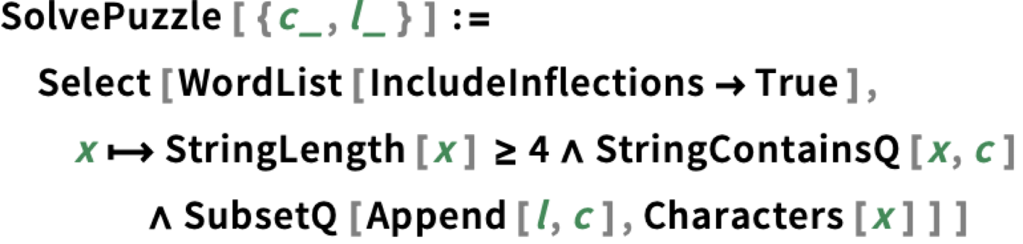
Of course, making code “elegant” is not just a question of formatting; it’s also a question of what’s actually in the code. And, yes, as with writing text, it takes effort to craft code that “expresses itself elegantly”. But the good news is that the Wolfram Language—through its uniquely broad and high-level character—makes it surprisingly straightforward to create code that expresses itself extremely elegantly.

But the point now is to make that code not only elegant in content, but also elegant in formatting. In technical documents it’s common to see math that’s at least formatted elegantly. But when one sees code, more often than not, it looks like something only a machine could appreciate. Of course, if the code is in a traditional programming language, it’ll usually be long and not really intended for human consumption. But what if it’s elegantly crafted Wolfram Language code? Well then we’d like it to look as attractive as text and math. And that’s the point of our Elegant Code project.

There are many tradeoffs, and many issues to be navigated. But in Version 13.3 we’re definitely making progress. Here’s an example that doesn’t have so many “words”, but where the elegant code formatting still makes the “blocking” of the code more obvious:

Here’s a slightly longer piece of code, where again the elegant code formatting helps pull out “readable” words, as well as making the overall structure of the code more obvious:

Particularly in recent years, we’ve added many mechanisms to let one write Wolfram Language that’s easier to read. There are the auto operator renderings, like m[[i]] turning into . And then there are things like the notation for pure functions. One particularly important element is Iconize, which lets you show any piece of Wolfram Language input in a visually “iconized” form—which nevertheless evaluates just like the corresponding underlying expression:

Iconize lets you effectively hide details (like large amounts of data, option settings, etc.) But sometimes you want to highlight things. You can do it with Style, Framed, Highlighted—and in Version 13.3, Squiggled:

By default, all these constructs persist through evaluation. But in Version 13.3 all of them now have the option StripOnInput, and with this set, you have something that shows up highlighted in an input cell, but where the highlighting is stripped when the expression is actually fed to the Wolfram Language kernel.

These show their highlighting in the notebook:

But when used in input, the highlighting is stripped:

See More Also…

A great strength of the Wolfram Language (yes, perhaps initiated by my original 1988 Mathematica Book) is its detailed documentation—which has now proved valuable not only for human users but also for AIs. Plotting the number of words that appear in the documentation in successive versions, we see a strong progressive increase:

Words graph

But with all that documentation, and all those new things to be documented, the problem of appropriately crosslinking everything has increased. Even back in Version 1.0, when the documentation was a physical book, there were “See Also’s” between functions:

Versioni 1.0 documentation

And by now there’s a complicated network of such See Also’s:

But that’s just the network of how functions point to functions. What about other kinds of constructs? Like formats, characters or entity types—or, for that matter, entries in the Wolfram Function Repository, Wolfram Data Repository, etc. Well, in Version 13.3 we’ve done a first iteration of crosslinking all these kinds of things.

So here now are the “See Also” areas for Graph and Molecule:

Graph see also options

Molecule see also options

Not only are there functions here; there are also other kinds of things that a person (or AI) looking at these pages might find relevant.

It’s great to be able to follow links, but sometimes it’s better just to have material immediately accessible, without following a link. Back in Version 1.0 we made the decision that when a function inherits some of its options from a “base function” (say Plot from Graphics), we only need to explicitly list the non-inherited option values. At the time, this was a good way to save a little paper in the printed book. But now the optimization is different, and finally in Version 13.3 we have a way to show “All Options”—tucked away so it doesn’t distract from the typically-more-important non-inherited options.

Here’s the setup for Plot. First, the list of non-inherited option values:

Plot non-inherited option values

Then, at the end of the Details section

Details and options

which opens to:

Expanded list of all options

Pictures from Words: Generative AI for Images

One of the remarkable things that’s emerged as a possibility from recent advances in AI and neural nets is the generation of images from textual descriptions. It’s not yet realistic to do this at all well on anything but a high-end (and typically server) GPU-enabled machine. But in Version 13.3 there’s now a built-in function ImageSynthesize that can get images synthesized, for now through an external API.

You give text, and ImageSynthesize will try to generate images for which that text is a description:

Sometimes these images will be directly useful in their own right, perhaps as “theming images” for documents or user interfaces. Sometimes they will provide raw material that can be developed into icons or other art. And sometimes they are most useful as inputs to tests or other algorithms.

And one of the important things about ImageSynthesize is that it can immediately be used as part of any Wolfram Language workflow. Pick a random sentence from Alice in Wonderland:

Now ImageSynthesize can “illustrate” it:

Or we can get AI to feed AI:

ImageSynthesize is set up to automatically be able to synthesize images of different sizes:

You can take the output of ImageSynthesize and immediately process it:

ImageSynthesize can not only produce complete images, but can also fill in transparent parts of “incomplete” images:

In addition to ImageSynthesize and all its new LLM functionality, Version 13.3 also includes a number of advances in the core machine learning system for Wolfram Language. Probably the most notable are speedups of up to 10x and beyond for neural net training and evaluation on x86-compatible systems, as well as better models for ImageIdentify. There are also a variety of new networks in the Wolfram Neural Net Repository, particularly ones based on transformers.

Digital Twins: Fitting System Models to Data

It’s been five years since we first began to introduce industrial-scale systems engineering capabilities in the Wolfram Language. The goal is to be able to compute with models of engineering and other systems that can be described by (potentially very large) collections of ordinary differential equations and their discrete analogs. Our separate Wolfram System Modeler product provides an IDE and GUI for graphically creating such models.

For the past five years we’ve been able to do high-efficiency simulation of these models from within the Wolfram Language. And over the past few years we’ve been adding all sorts of higher-level functionality for programmatically creating models, and for systematically analyzing their behavior. A major focus in recent versions has been the synthesis of control systems, and various forms of controllers.

Version 13.3 now tackles a different issue, which is the alignment of models with real-world systems. The idea is to have a model which contains certain parameters, and then to determine these parameters by essentially fitting the model’s behavior to observed behavior of a real-world system.

Let’s start by talking about a simple case where our model is just defined by a single ODE:

This ODE is simple enough that we can find its analytical solution:

So now let’s make some “simulated real-world data” assuming a = 2, and with some noise:

Here’s what the data looks like:

Now let’s try to “calibrate” our original model using this data. It’s a process similar to machine learning training. In this case we make an “initial guess” that the parameter a is 1; then when SystemModelCalibrate runs it shows the “loss” decreasing as the correct value of a is found:

The “calibrated” model does indeed have a ≈ 2:

Now we can compare the calibrated model with the data:

As a slightly more realistic engineering-style example let’s look at a model of an electric motor (with both electrical and mechanical parts):

Let’s say we’ve got some data on the behavior of the motor; here we’ve assumed that we’ve measured the angular velocity of a component in the motor as a function of time. Now we can use this data to calibrate parameters of the model (here the resistance of a resistor and the damping constant of a damper):

Here are the fitted parameter values:

And here’s a full plot of the angular velocity data, together with the fitted model and its 95% confidence bands:

SystemModelCalibrate can be used not only in fitting a model to real-world data, but also for example in fitting simpler models to more complicated ones, making possible various forms of “model simplification”.

Symbolic Testing Framework

The Wolfram Language is by many measures one of the world’s most complex pieces of software engineering. And over the decades we’ve developed a large and powerful system for testing and validating it. A decade ago—in Version 10—we began to make some of our internal tools available for anyone writing Wolfram Language code. Now in Version 13.3 we’re introducing a more streamlined—and “symbolic”—version of our testing framework.

The basic idea is that each test is represented by a symbolic TestObject, created using TestCreate:

On its own, TestObject is an inert object. You can run the test it represents using TestEvaluate:

Each test object has a whole collection of properties, some of which only get filled in when the test is run:

It’s very convenient to have symbolic test objects that one can manipulate using standard Wolfram Language functions, say selecting tests with particular features, or generating new tests from old. And when one builds a test suite, one does it just by making a list of test objects.

This makes a list of test objects (and, yes, there’s some trickiness because TestCreate needs to keep unevaluated the expression that’s going to be tested):

But given these tests, we can now generate a report from running them:

TestReport has various options that allow you to monitor and control the running of a test suite. For example, here we’re saying to echo every "TestEvaluated" event that occurs:

Did You Get That Math Right?

Most of what the Wolfram Language is about is taking inputs from humans (as well as programs, and now AIs) and computing outputs from them. But a few years ago we started introducing capabilities for having the Wolfram Language ask questions of humans, and then assessing their answers.

In recent versions we’ve been building up sophisticated ways to construct and deploy “quizzes” and other collections of questions. But one of the core issues is always how to determine whether a person has answered a particular question correctly. Sometimes that’s easy to determine. If we ask “What is 2 + 2?”, the answer better be “4” (or conceivably “four”). But what if we ask a question where the answer is some algebraic expression? The issue is that there may be many mathematically equal forms of that expression. And it depends on what exactly one’s asking whether one considers a particular form to be the “right answer” or not.

For example, here we’re computing a derivative:

And here we’re doing a factoring problem:

These two answers are mathematically equal. And they’d both be “reasonable answers” for the derivative if it appeared as a question in a calculus course. But in an algebra course, one wouldn’t want to consider the unfactored form a “correct answer” to the factoring problem, even though it’s “mathematically equal”.

And to deal with these kinds of issues, we’re introducing in Version 13.3 more detailed mathematical assessment functions. With a "CalculusResult" assessment function, it’s OK to give the unfactored form:

But with a "PolynomialResult" assessment function, the algebraic form of the expression has to be the same for it to be considered “correct”:

There’s also another type of assessment function—"ArithmeticResult"—which only allows trivial arithmetic rearrangements, so that it considers 2 + 3 equivalent to 3 + 2, but doesn’t consider 2/3 equivalent to 4/6:

Here’s how you’d build a question with this:

And now if you type “2/3” it’ll say you’ve got it right, but if you type “4/6” it won’t. However, if you use, say, "CalculusResult" in the assessment function, it’ll say you got it right even if you type “4/6”.

Streamlining Parallel Computation

Ever since the mid-1990s there’s been the capability to do parallel computation in the Wolfram Language. And certainly for me it’s been critical in a whole range of research projects I’ve done. I currently have 156 cores routinely available in my “home” setup, distributed across 6 machines. It’s sometimes challenging from a system administration point of view to keep all those machines and their networking running as one wants. And one of the things we’ve been doing in recent versions—and now completed in Version 13.3—is to make it easier from within the Wolfram Language to see and manage what’s going on.

It all comes down to specifying the configuration of kernels. And in Version 13.3 that’s now done using symbolic KernelConfiguration objects. Here’s an example of one:

There’s all sorts of information in the kernel configuration object:

It describes “where” a kernel with that configuration will be, how to get to it, and how it should be launched. The kernel might just be local to your machine. Or it might be on a remote machine, accessible through ssh, or https, or our own wstp (Wolfram Symbolic Transport Protocol) or lwg (Lightweight Grid) protocols.

In Version 13.3 there’s now a GUI for setting up kernel configurations:

Kernel configuration editor

The Kernel Configuration Editor lets you enter all the details that are needed, about network connections, authentication, locations of executables, etc.

But once you’ve set up a KernelConfiguration object, that’s all you ever need—for example to say “where” to do a remote evaluation:

ParallelMap and other parallel functions then just work by doing their computations on kernels specified by a list of KernelConfiguration objects. You can set up the list in the Kernels Settings GUI:

Parallel kernels settings

Here’s my personal default collection of parallel kernels:

This now counts the number of individual kernels running on each machine specified by these configurations:

In Version 13.3 a convenient new feature is named collections of kernels. For example, this runs a single “representative” kernel on each distinct machine:

Just Call That C Function! Direct Access to External Libraries

Let’s say you’ve got an external library written in C—or in some other language that can compile to a C-compatible library. In Version 13.3 there’s now foreign function interface (FFI) capability that allows you to directly call any function in the external library just using Wolfram Language code.

Here’s a very trivial C function:

Trivial C function

This function happens to be included in compiled form in the compilerDemoBase library that’s part of Wolfram Language documentation. Given this library, you can use ForeignFunctionLoad to load the library and create a Wolfram Language function that directly calls the C addone function. All you need do is specify the library and C function, and then give the type signature for the function:

Now ff is a Wolfram Language function that calls the C addone function:

The C function addone happens to have a particularly simple type signature, that can immediately be represented in terms of compiler types that have direct analogs as Wolfram Language expressions. But in working with low-level languages, it’s very common to have to deal directly with raw memory, which is something that never happens when you’re purely working at the Wolfram Language level.

So, for example, in the OpenSSL library there’s a function called RAND_bytes, whose C type signature is:

RAND_bytes

And the important thing to notice is that this contains a pointer to a buffer buf that gets filled by RAND_bytes. If you were calling RAND_bytes from C, you’d first allocate memory for this buffer, then—after calling RAND_bytes—read back whatever was written to the buffer. So how can you do something analogous when you’re calling RAND_bytes using ForeignFunction in Wolfram Language? In Version 13.3 we’re introducing a family of constructs for working with pointers and raw memory.

So, for example, here’s how we can create a Wolfram Language foreign function corresponding to RAND_bytes:

But to actually use this, we need to be able to allocate the buffer, which in Version 13.3 we can do with RawMemoryAllocate:

This creates a buffer that can store 10 unsigned chars. Now we can call rb, giving it this buffer:

rb will fill the buffer—and then we can import the results back into Wolfram Language:

There’s some complicated stuff going on here. RawMemoryAllocate does ultimately allocate raw memory—and you can see its hex address in the symbolic object that’s returned. But RawMemoryAllocate creates a ManagedObject, which keeps track of whether it’s being referenced, and automatically frees the memory that’s been allocated when nothing references it anymore.

Long ago languages like BASIC provided PEEK and POKE functions for reading and writing raw memory. It was always a dangerous thing to do—and it’s still dangerous. But it’s somewhat higher level in Wolfram Language, where in Version 13.3 there are now functions like RawMemoryRead and RawMemoryWrite. (For writing data into a buffer, RawMemoryExport is also relevant.)

Most of the time it’s very convenient to deal with memory-managed ManagedObject constructs. But for the full low-level experience, Version 13.3 provides UnmanageObject, which disconnects automatic memory management for a managed object, and requires you to explicitly use RawMemoryFree to free it.

One feature of C-like languages is the concept of a function pointer. And normally the function that the pointer is pointing to is just something like a C function. But in Version 13.3 there’s another possibility: it can be a function defined in Wolfram Language. Or, in other words, from within an external C function it’s possible to call back into the Wolfram Language.

Let’s use this C program:

C program

You can actually compile it right from Wolfram Language using:

Now we load frun as a foreign function—with a type signature that uses "OpaqueRawPointer" to represent the function pointer:

What we need next is to create a function pointer that points to a callback to Wolfram Language:

The Wolfram Language function here is just Echo. But when we call frun with the cbfun function pointer we can see our C code calling back into Wolfram Language to evaluate Echo:

ForeignFunctionLoad provides an extremely convenient way to call external C-like functions directly from top-level Wolfram Language. But if you’re calling C-like functions a great many times, you’ll sometimes want to do it using compiled Wolfram Language code. And you can do this using the LibraryFunctionDeclaration mechanism that was introduced in Version 13.1. It’ll be more complicated to set up, and it’ll require an explicit compilation step, but there’ll be slightly less “overhead” in calling the external functions.

The Advance of the Compiler Continues

For several years we’ve had an ambitious project to develop a large-scale compiler for the Wolfram Language. And in each successive version we’re further extending and enhancing the compiler. In Version 13.3 we’ve managed to compile more of the compiler itself (which, needless to say, is written in Wolfram Language)—thereby making the compiler more efficient in compiling code. We’ve also enhanced the performance of the code generated by the compiler—particularly by optimizing memory management done in the compiled code.

Over the past several versions we’ve been steadily making it possible to compile more and more of the Wolfram Language. But it’ll never make sense to compile everything—and in Version 13.3 we’re adding KernelEvaluate to make it more convenient to call back from compiled code to the Wolfram Language kernel.

Here’s an example:

We’ve got an argument n that’s declared as being of type MachineInteger. Then we’re doing a computation on n in the kernel, and using TypeHint to specify that its result will be of type MachineInteger. There’s at least arithmetic going on outside the KernelEvaluate that can be compiled, even though the KernelEvaluate is just calling uncompiled code:

There are other enhancements to the compiler in Version 13.3 as well. For example, Cast now allows data types to be cast in a way that directly emulates what the C language does. There’s also now SequenceType, which is a type analogous to the Wolfram Language Sequence construct—and able to represent an arbitrary-length sequence of arguments to a function.

And Much More…

In addition to everything we’ve already discussed here, there are lots of other updates and enhancements in Version 13.3—as well as thousands of bug fixes.

Some of the additions fill out corners of functionality, adding completeness or consistency. Statistical fitting functions like LinearModelFit now accept input in all various association etc. forms that machine learning functions like Classify accept. TourVideo now lets you “tour” GeoGraphics, with waypoints specified by geo positions. ByteArray now supports the “corner case” of zero-length byte arrays. The compiler can now handle byte array functions, and additional string functions. Nearly 40 additional special functions can now handle numeric interval computations. BarcodeImage adds support for UPCE and Code93 barcodes. SolidMechanicsPDEComponent adds support for the Yeoh hyperelastic model. And—twenty years after we first introduced export of SVG, there’s now built-in support for import of SVG not only to raster graphics, but also to vector graphics.

There are new “utility” functions like RealValuedNumberQ and RealValuedNumericQ. There’s a new function FindImageShapes that begins the process of systematically finding geometrical forms in images. There are a number of new data structures—like "SortedKeyStore" and "CuckooFilter".

There are also functions whose algorithms—and output—have been improved. ImageSaliencyFilter now uses new machine-learning-based methods. RSolveValue gives cleaner and smaller results for the important case of linear difference equations with constant coefficients.

🔲 ☆

Introducing Chat Notebooks: Integrating LLMs into the Notebook Paradigm

This is part of an ongoing series about our LLM-related technology:ChatGPT Gets Its “Wolfram Superpowers”!Instant Plugins for ChatGPT: Introducing the Wolfram ChatGPT Plugin KitThe New World of LLM Functions: Integrating LLM Technology into the Wolfram LanguagePrompts for Work & Play: Launching the Wolfram Prompt RepositoryIntroducing Chat Notebooks: Integrating LLMs into the Notebook Paradigm

Introducing Chat Notebooks: Integrating LLMs into the Notebook Paradigm

A New Kind of Notebook

We originally invented the concept of “Notebooks” back in 1987, for Version 1.0 of Mathematica. And over the past 36 years, Notebooks have proved to be an incredibly convenient medium in which to do—and publish—work (and indeed, I, for example, have created hundreds of thousands of them). And, yes, eventually the basic concepts of Notebooks were widely copied—though still not even with everything we had back in 1987!

Well, now there’s a new challenge and opportunity for Notebooks: integrating LLM functionality into them. It’s an interesting design problem, and I’m pretty pleased with what we’ve come up with. And today we’re introducing Chat Notebooks as a new kind of Notebook that supports LLM-based chat functionality.

The functionality described here will be built into the upcoming version of Wolfram Language (Version 13.3). To install it in the now-current version (Version 13.2), use

PacletInstall["Wolfram/Chatbook"]

and

PacletInstall["Wolfram/LLMFunctions"].

You will also need an API key for the OpenAI LLM or another LLM.

Just as with ordinary Notebooks, there are many ways to use Chat Notebooks. One that I’m particularly excited about—especially because of its potential to open up computational language to so many people—is for providing interactive Wolfram Language assistance. But I’ll talk about that separately. And instead here I’ll concentrate on the (already very rich) general concept of Chat Notebooks.

The basic idea is simple: there’s a new kind of cell—a chat cell—that communicates with an LLM. (In what we’re calling “Chat-Driven Notebooks” chat cells are the default; in “Chat-Enabled Notebooks” you get a chat cell by pressing '—i.e. quote—when you first create the cell.)


In a standard Notebook, we’re used to having input cells containing Wolfram Language, together with output cells that give the results from evaluating that Wolfram Language input:

And at a basic level, a chat cell is just a type of cell that uses an LLM—rather than the Wolfram Language kernel—to “evaluate” its output. And indeed, in a Chat Notebook, the way you send your input to the LLM is to press shiftenter, just like for Wolfram Language input.

And just like for standard input and output cells, chat input and output cells are grouped, so you can select them together, or double-click one of them to open or close them:

Opening and closing cells

One immediate difference with chat cells is that whereas an ordinary output cell is produced all at once, the contents of a chat output cell progressively “stream in” a word (or so) at a time, as the LLM generates it.

There’s another important difference too. In an ordinary Notebook there’s a “temporal thread of evaluation” in which inputs and outputs appear in the sequence they’re generated in time (as indicated by In[n] and Out[n], quite independent of where they are placed in the Notebook. Thus, for example, if you evaluate x = 5 in an input cell, then subsequently ask for the value of x, the result will be 5 wherever in the notebook you ask—even if it’s above the “x = 5” cell:

x = 5 calculations

But with chat cells it’s a different story. Now the order of cells in the Notebook matters. The “thread of a chat” is determined not by when chat cells were evaluated, but instead by the order in which they appear in the notebook.

Order of chat cells in thread

Going down the notebook, successive chat cells are “aware” of what’s in cells above them. But even if we add it later, a cell placed at the top won’t “know about” anything in cells below it.

All of this reflects an important difference between ordinary Wolfram Language evaluation and “LLM evaluation”. In Wolfram Language evaluation, the Wolfram Language kernel always has an internal state, and whatever you do in the notebook is in a sense merely a window into that state. But for LLM evaluation the whole state is determined by the actual content of the notebook.

And each time you do an LLM evaluation, the Notebook system will package up all the content above the cell in which you’re doing the evaluation, and send it to the LLM. The LLM in a sense never knows anything about time history; all it knows is what’s in the notebook when the LLM evaluation is done.

There are many consequences of this. One is that you can edit the chat history and “reevaluate with new history”. When the reevaluation “overwrites” a cell, the Chat Notebook will maintain the older version, and you can get back to it by pressing the arrows (for purposes of LLM evaluation, the chat history is always considered to be what’s showing when you do the evaluation):

LLM evaluations pick up content that appears above them in the notebook. But there’s an important way to limit this, and to separate or “modularize” chats: the idea of a chatblock.

You can begin a chatblock by pressing ~ (tilde) when you create a cell in the Notebook you’ll then get:

Chatblock separator

And the point is that this indicates the beginning of a new chat. When you evaluate a chat cell below this separator, it’ll only use content up to the separator—so that means that in a single Chat Notebook, you can have any number of independent “chat sessions”, delimited by chatblock separators:

Name chat

In a sense LLM evaluation is a very Notebook-centric form of evaluation, always based on the sequence of content that appears in the Notebook. As we’ll discuss below, there are different detailed forms of LLM evaluation, but in most cases the evaluation will operate not just on chat cells, but on all cells that appear above it in a given chatblock.

Another difference from ordinary evaluation is that LLM evaluation can often not be repeatable. Yes, if there are random numbers, or external inputs, ordinary Wolfram Language evaluation may not be repeatable. But the core evaluation process in Wolfram Language is completely repeatable. In an LLM, however, that may not be the case. For example, particularly if the LLM is operated with a nonzero value of its “temperature” parameter (which is usually the default), it’s pretty much guaranteed to give different results every time an evaluation is done.

And in using Chat Notebooks, it’ll sometimes be convenient to just try to evaluate a chat cell multiple times until you get what you want. (You can go between different choices using the arrows.) Another helpful “trick” in Chat Notebooks is to edit not just your input, but also the output generated from LLM evaluation. When you do an LLM evaluation, the LLM is just given whatever appears above in the Notebook, regardless of where that “came from”. So if the LLM “makes a mistake” you can just fix it yourself, and then the LLM will typically “pick up the fix” when it comes to do later evaluations.

The default in Chat Notebooks is always to use previous cells as “context” for any chat input you provide. But there’s also a mechanism for having “side chats” that don’t use (or affect) context. Instead of just typing to get a chat cell (in a Chat-Driven Notebook), start the cell with ' (“quote”) to get a “side chat” cell (in a Chat-Enabled Notebook, it’s ' to get a chat cell, and '' to get a side chat cell):

Side chat cell

Who Are You Gonna Talk To?

When you evaluate a chat cell, you’ll get a response from an LLM. But what determines the “persona” that’ll be used for the LLM—or in general how the LLM is configured? There are multiple levels at which this can be specified—from overall Preference settings to Chat Notebook settings to chatblocks to individual chat cells.

For a chatblock, for example, click the little chat icon to the left and you’ll see a menu of possible personas:

Personas menu

Pick a particular persona and its icon will show up “perched” on the chatblock separator—and then in every chat cell that follows it’ll be that persona that by default responds to you:

Birdnardo query

You can tell it’s that persona responding because its icon will show up as the “label” for the response. (It’ll also appear next to your input if you hover over the chat cell icon).

We mentioned in passing above that when there are two kinds of Chat Notebooks you can create (e.g. with the File > New menu): Chat-Enabled Notebooks and Chat-Driven Notebooks. In future versions of the Wolfram Notebook system, Chat-Enabled Notebooks will probably be the standard default for all new notebooks, but for now it’s something you have to explicitly choose.

So what is a Chat-Enabled Notebook, and how is it different from a Chat-Driven Notebook? The basic point is that a Chat-Enabled Notebook is intended to be used just like Wolfram Notebooks have been used for 35 years—but with additional chat capabilities added. In a Chat-Enabled Notebook the default new cell type (assuming you’re using the default stylesheet) expects Wolfram Language input. To get a chat cell, you explicitly type ' (“quote”) at the beginning of the cell. And when you make that chat cell, it’ll by default be talking to the Code Assistant persona, ready to help you with generating Wolfram Language code.

A Chat-Driven Notebook is something different: it’s a notebook where chats are the primary content—and by default new cells are always chat cells, and there’s no particular expectation that you’ll be talking about things to do with Wolfram Language. There’s no special persona by default in Chat-Driven Notebook, and instead one’s pretty much just talking to the generic LLM (though there’s some additional prompting about being used in a Notebook, etc.)

If you want to talk to another persona, though, you can specify that in the menu of personas. There are a few personas listed by default. But there are many more in the Wolfram Prompt Repository. And from Add & Manage Personas you can open the personas section of the Prompt Repository:

Wolfram Prompt Repository personas

Then you can go to a persona page, and press the Install button to install that persona in your session:

GenZSpeak persona

Now you’ll be able to select this persona from any chatblock, chat cell, etc. persona menu:

GenZSpeak chat

The Wolfram Prompt Repository contains a growing selection of curated contributed personas. But the Install from URL menu item also lets you install personas that have been independently deployed (for example in the Wolfram Cloud), and are available either publicly or for specific users. (As discussed elsewhere, you can create personas using a Prompt Resource Definition Notebook.)

Given a named persona—either defined in the Wolfram Prompt Repository, or that you’ve explicitly installed—you can always “direct chat” that persona in a particular chat cell by using @persona:

Chat query about feathers

When you direct chat a persona in a particular chat cell, that persona gets sent the whole previous history in your current chatblock. But after that persona has responded, subsequent chat cells revert to using the current default persona. Nevertheless, any persona that you direct chat will automatically get installed in the list of personas you can use. Note, by the way, that direct chatting is an independent idea from side chats. Side chats don’t by default affect what persona you’re talking to, but give you a “localized” context, while direct chats affect the persona you’re talking to, but are “flowed into” the global history of the current chatblock.

Personas let you define all sorts of aspects of how you want an LLM to behave. But ultimately you also have to define the underlying LLM itself. What model should it use? With what “temperature”? etc. At the bottom of the same menus that list personas there’s an Advanced Settings item:

Advanced Settings menu

Like personas, these can be set at a chat cell level, chatblock level, notebook level—or globally, through Preferences settings. It’s typical to define things like authentication at the Preferences level. And ultimately everything about the configuration of an LLM is specified by a symbolic LLMConfiguration object.

As we’ll discuss elsewhere, a very important additional feature of full LLMConfiguration objects is that they can specify “tools” that should be available to an LLM—essentially Wolfram Language APIs that the LLM should be able to send requests to in order to get computational results or computational actions.

Within a particular Wolfram Language session, you can specify a default LLM configuration by setting the value of $LLMEvaluator. You can also programmatically create a Chat Notebook with a specified LLM configuration using:

(This will make a chat-driven notebook; you can use "ChatEnabled" to make a chat-enabled notebook.)

Applying Functions in a Chat Notebook

As we discussed elsewhere, personas are ultimately just prompts. So when, for example, we say @Yoda we’re really just adding the “Yoda prompt” (i.e. LLMPrompt["Yoda"]) into a chat evaluation.

But there are all sorts of prompts that don’t correspond to what we’d normally think of as personas. For example, there are “modifier prompts”, like Emojified or SEOptimize or TweetConvert, that describe particular output we want to get. And in a Chat Notebook, we can add such modifier prompts just using #prompt:

HaikuStyled chat modifier

The reason this works is that “under the hood”, a chat evaluation is effectively LLMSynthesize["input"], and adding either a persona or a modifier prompt is achieved with LLMSynthesize[LLMPrompt[]].

You can add more than one modifier prompt just by putting in multiple # items. But what if a modifier prompt has a “parameter”, like in the case of "LLMPrompt["Translated", "French"]"? Chat Notebooks provide a syntax for that, with each parameter separated by |, as in #prompt|parameter:

HaikuStyled and Translated chat modifiers

Personas and modifiers are both intended to affect the output generated by an LLM in a chat. But the Wolfram Prompt Repository also contains “function prompts”, that are intended to operate on a specific piece of input you give. Function prompts are particularly suitable for programmatic use, as in:

But it’s also possible to use function prompts in Chat Notebooks. !prompt specifies a function prompt:

FormalRephrase chat function prompt

By default, a function prompt in a chat cell takes as its input the text you explicitly give in the chat cell (though it still “sees” previous history in the current chatblock.) But it’s also common to want to put the input in a cell of its own. You can make a function prompt take its input from the previous cell in the notebook by using !prompt^:

FormalRephrase example

But what if you want to feed the complete history (in the current chatblock) to a function prompt? You can do that by using ^^ instead of ^:

Additional FormalRephrase example

And, yes, there are a lot of little notations in Chat Notebooks. One gets used to them quickly, but here—for convenience—are all of them collected in a table:

Chat Notebooks notation menu

The Design of Chat Notebooks

One of the great long-term strengths of the Wolfram Language is the coherence of its design. And that design coherence extends not only across the language itself, but also to the whole system around the language, including Wolfram Notebooks. So what about Chat Notebooks? As we said above, Chat Notebooks represent a new kind of Notebook—that have new kinds of requirements, and bring new design challenges. But as has happened so many times before, the whole Wolfram Language and Notebook paradigm turns out to be strong and general enough that we’ve been able to design Chat Notebooks so they fit coherently in with the rest of the system. And particularly for those (humans and AIs!) who know the existing system, it may be helpful to discuss some of the precedents and analogies for Chat Notebooks that exist elsewhere in the system.

A key feature of Chat Notebooks is the concept of using a different evaluator for certain notebook content—in their case, an LLM evaluator for chat cells. But it turns out that the idea of having different evaluators is something that’s been around ever since we first invented Notebooks 36 years ago. Back in those days a common setup was a Notebook “front end” that could send evaluations either to a kernel running on your local machine, or to remote kernels running on other (perhaps more powerful) machines. (And, yes, there were shades of what we’d now call “the cloud”, though in those days remote computers often had phone connections, etc.)

Right from the beginning we discussed having evaluators that weren’t directly based on what’s now Wolfram Language (and indeed at a programmatic level we provided plenty of access to external programs, etc.). But it was only when we released Wolfram|Alpha in 2009 that we finally had a compelling reason to think about integrating something other than Wolfram Language evaluation into the core user interface of Notebooks. Because then—through Wolfram|Alpha’s natural language understanding capabilities—we had a way to specify Wolfram Language computations using something other than Wolfram Language: ordinary natural language.

So this led us to introduce Wolfram|Alpha cells—where evaluation first interprets natural language you type, then does the Wolfram Language computation it specifies. You get a Wolfram|Alpha cell by pressing = when you create the cell (we also introduced the inline control= mechanism); then shiftenter does the evaluation:

Wolfram|Alpha cell

In 2017 (with Version 11.2) the notion of access to “other evaluators” from notebooks took another step—with the introduction of external evaluation cells:

External evaluation cell

And with this also came the notion of a menu of “possible evaluators”—a precursor to the personas menu of Chat Notebooks:

External software menu

Then in 2019 came the introduction of Wolfram|Alpha Notebook Edition, with its whole framework around natural language “Wolfram|Alpha-style” input cells:

Wolfram|Alpha Notebook Edition input cells

And in a sense this was the most direct precursor to Chat Notebooks. But now instead of having “free-form input” cells going to Wolfram|Alpha, we have chat cells going to an LLM.

At a programmatic level, ChatEvaluate (and LLMSynthesize) are in many ways not so different from CloudEvaluate, RemoteEvaluate or ParallelEvaluate. But what’s new is the Notebook interface aspect—which is what we’ve invented Chat Notebooks for. In things like ExternalEvaluate and ParallelEvaluate there’s a state maintained within the evaluator. But Wolfram|Alpha, for example, is typically stateless. So in Wolfram|Alpha Notebook Edition “state” is determined from previous cells in the notebook—which is essentially the same mechanism used in Chat Notebooks.

But one of the new things in Chat Notebooks is that not only are previous cells that are somehow identified as “input” used to determine the “state”, but other cells (like text cells) are used as well. And, yes, ever since Version 3 in 1996, there’ve been notebook programming constructs that have been able to process arbitrary notebook content. But Chat Notebooks are the first time “non-input” has been used in “evaluation”.

Most of the defining features of Notebooks—like cells, cell groups, evaluation behavior, and so on—have been there ever since the beginning, back in 1988. But gradually over the years, we’ve progressively polished the concepts of Notebooks—introducing ideas like reverse-closed cells, template boxes, input ligatures, etc. And what’s remarkable to see now is how Chat Notebooks build on all these concepts.

You can cut, copy, paste chat cells just like any other kinds of cells. You can close chat outputs, or reverse close chat inputs. It’s all the same as in the Notebook paradigm we’ve had for so long. But there are new ideas, like alternate outputs, chatblocks, etc. And no doubt over the months and years to come—as we see just how Chat Notebooks are used—we’ll invent ways to extend and polish the Chat Notebook experience. But as of now, it’s exciting to see how we’ve been able to take the paradigm that we invented more than 35 years ago and use it to deliver such a rich and powerful interface to those most modern of things: LLMs.

🔲 ☆

The New World of LLM Functions: Integrating LLM Technology into the Wolfram Language

This is part of an ongoing series about our LLM-related technology:ChatGPT Gets Its “Wolfram Superpowers”!Instant Plugins for ChatGPT: Introducing the Wolfram ChatGPT Plugin KitThe New World of LLM Functions: Integrating LLM Technology into the Wolfram LanguagePrompts for Work & Play: Launching the Wolfram Prompt RepositoryIntroducing Chat Notebooks: Integrating LLMs into the Notebook Paradigm

The New World of LLM Functions: Integrating LLM Technology into the Wolfram Language

Turning LLM Capabilities into Functions

So far, we mostly think of LLMs as things we interact directly with, say through chat interfaces. But what if we could take LLM functionality and “package it up” so that we can routinely use it as a component inside anything we’re doing? Well, that’s what our new LLMFunction is about.

The functionality described here will be built into the upcoming version of Wolfram Language (Version 13.3). To install it in the now-current version (Version 13.2), use

PacletInstall["Wolfram/LLMFunctions"].

You will also need an API key for the OpenAI LLM or another LLM.

Here’s a very simple example—an LLMFunction that rewrites a sentence in active voice:

Here’s another example—an LLMFunction with three arguments, that finds word analogies:

And here’s one more example—that now uses some “everyday knowledge” and “creativity”:

In each case here what we’re doing is to use natural language to specify a function, that’s then implemented by an LLM. And even though there’s a lot going on inside the LLM when it evaluates the function, we can treat the LLMFunction itself in a very “lightweight” way, using it just like any other function in the Wolfram Language.

Ultimately what makes this possible is the symbolic nature of the Wolfram Language—and the ability to represent any function (or, for that matter, anything else) as a symbolic object. To the Wolfram Language 2 + 3 is Plus[2,3], where Plus is just a symbolic object. And for example doing a very simple piece of machine learning, we again get a symbolic object

which can be used as a function and applied to an argument to get a result:

And so it is with LLMFunction. On its own, LLMFunction is just a symbolic object (we’ll explain later why it’s displayed like this):

But when we apply it to an argument, the LLM does its work, and we get a result:

If we want to, we can assign a name to the LLMFunction

and now we can use this name to refer to the function:

It’s all rather elegant and powerful—and connects quite seamlessly into the whole structure of the Wolfram Language. So, for example, just as we can map a symbolic object f over a list

so now we can map LLMFunction over a list:

And just as we can progressively nest f

so now we can progressively nest an LLMFunctionhere producing a “funnier and funnier” version of a sentence:

We can similarly use Outer

to produce an array of LLMFunction results:

It’s remarkable what becomes possible when one integrates LLMs with the Wolfram Language. One thing one can do is take results of Wolfram Language computations (here a very simple one) and feed them into an LLM:

We can also just directly feed in data:

But now we can take this textual output and apply another LLMFunction to it (% stands for the last output):

And then perhaps yet another LLMFunction:

If we want, we can compose these functions together (f@x is equivalent to f[x]):

As another example, let’s generate some random words:

Now we can use these as “input data” for an LLMFunction:

The input for an LLMFunction doesn’t have to be “immediately textual”:

By default, though, the output from LLMFunction is purely textual:

But it doesn’t have to be that way. By giving a second argument to LLMFunction you can say you want actual, structured computable output. And then through a mixture of “LLM magic” and natural language understanding capabilities built into the Wolfram Language, the LLMFunction will attempt to interpret output so it’s given in a specified, computable form.

For example, this gives output as actual Wolfram Language colors:

And here we’re asking for output as a Wolfram Language "City" entity:

Here’s a slightly more elaborate example where we ask for a list of cities:

And, of course, this is a computable result, that we can for example immediately plot:

Here’s another example, again tapping the “common-sense knowledge” of the LLM:

Now we can immediately use this LLMFunction to sort objects in decreasing order of size:

An important use of LLM functions is in extracting structured data from text. Imagine we have the text:

Now we can start asking questions—and getting back computable answers. Let’s define:

Now we can “ask a quantity question” based on that text:

And we can go on, getting back structured data, and computing with it:

There’s often a lot of “common sense” involved. Like here the LLM has to “figure out” that by “mass” we mean “body weight”:

Here’s another sample piece of text:

And once again we can use LLMFunction to ask questions about it, and get back structured results:

There’s a lot one can do with LLMFunction. Here’s an example of an LLMFunction for writing Wolfram Language:

The result is a string. But if we’re brave, we can turn it into an expression, which will immediately be evaluated:

Here’s a “heuristic conversion function”, where we’ve bravely specified that we want the result as an expression:

Functions from Examples

LLMs—like typical neural nets—are built by learning from examples. Initially those examples include billions of webpages, etc. But LLMs also have an uncanny ability to “keep on learning”, even from very few examples. And LLMExampleFunction makes it easy to give examples, and then have the LLM apply what it’s learned from them.

Here we’re giving just one example of a simple structural rearrangement, and—rather remarkably—the LLM successfully generalizes this and is immediately able to do the “correct” rearrangement in a more complicated case:

Here we’re again giving just one example—and the LLM successfully figures out to sort in numerical order, with letters before numbers:

LLMExampleFunction is pretty good at picking up on “typical things one wants to do”:

But sometimes it’s not quite sure what’s wanted:

Here’s another case where the LLM gives a good result, effectively also pulling in some general knowledge (of the meaning of ♂ and ♀):

One powerful way to use LLMExampleFunction is in converting between formats. Let’s say we produce the following output:

But instead of this “ASCII art”-like rendering, we want something that can immediately be given as input to Wolfram Language. What LLMExampleFunction lets us do is give one or more examples of what transformation we want to do. We don’t have to write a program that does string manipulation, etc. We just have to give an example of what we want, and then in effect have the LLM “generalize” to all the cases we need.

Let’s try a single example, based on how we’d like to transform the first “content line” of the output:

And, yes, this basically did what we need, and it’s straightforward to get it into a final Wolfram Language form:

So far we’ve just seen LLMExampleFunction doing essentially “structure-based” operations. But it can also do more “meaning-based” ones:

Often one ends up with something that can be thought of as an “analogy question”:

When it comes to more computational situations, it can do OK if one’s asking about things which are part of the corpus of “common-sense computational knowledge”:

But if there’s “actual computation” involved, it typically fails (the right answer here is 5! + 5 = 125):

Sometimes it’s hard for LLMExampleFunction to figure out what you want just from examples you give. Here we have in mind finding animals of the same color—but LLMExampleFunction doesn’t figure that out:

But if we add a “hint”, it’ll nail it:

We can think of LLMExampleFunction as a kind of textual analog of Predict. And, like Predict, LLMExampleFunction can take also examples in an all-inputs → all-outputs form:

Pre-written Prompts and the Wolfram Prompt Repository

So far we’ve been talking about creating LLM functions “from scratch”, in effect by explicitly writing out a “prompt” (or, alternatively, giving examples to learn from). But it’s often convenient to use—or at least include—“pre-written” prompts, either ones that you’ve created and stored before, or ones that come from our new Wolfram Prompt Repository:

Wolfram Prompt Repository

Other posts in this series will talk in more detail about the Wolfram Prompt Repository—and about how it can be used in things like Chat Notebooks. But here we’re going to talk about how it can be used “programmatically” for LLM functions.

The first approach is to use what we call “function prompts”—that are essentially pre-built LLMFunction objects. There’s a whole section of function prompts in the Prompt Repository. As one example, let’s consider the "Emojify" function prompt. Here’s its page in the Prompt Repository:

Emojify page

You can take any function prompt and apply it to specific text using LLMResourceFunction. Here’s what happens with the "Emojify" prompt:

And if you look at the pure result from LLMResourceFunction, we can see that it’s just an LLMFunction—whose content was obtained from the Prompt Repository:

Here’s another example:

And here we’re applying two different (but, in this particular case, approximately inverse) LLM functions from the Prompt Repository:

LLMResourceFunction can take more than one argument:

Something that we see here is that LLMResourceFunction can have an interpreter built into it—so that instead of just returning a string, it can return a computable (here held) Wolfram Language expression. So, for example, the "MovieSuggest" prompt in the Prompt Repository is defined to include an interpreter that gives "Movie" entities

from which we can do further computations, like:

Besides “function prompts”, another large section of the Prompt Repository is devoted to “persona” prompts. These are primarily intended for chats (“talk to a particular persona”), but they can also be used “programmatically” through LLMResourceFunction to ask for a single response “from the persona” to a particular input:

Beyond function and persona prompts, there’s a third major kind of prompt—that we call a “modifier prompt”—that’s intended to modify output from the LLM. An example of a modifier prompt is "ELI5" (“Explain Like I’m 5”). To “pull in” such a modifier prompt from the Prompt Repository, we use the general function LLMPrompt.

Say we’ve got an LLMFunction set up:

To modify it with "ELI5", we just insert LLMPrompt["ELI5"] into the “body” of the LLMFunction:

You can include multiple modifier prompts; some modifier prompts (like "Translated") are set up to “take parameters” (here, the language to have the output translated into):

We’ll talk later in more detail about how this works. But the basic idea is just that LLMPrompt retrieves representations of prompts from the Prompt Repository:

An important kind of modifier prompts are ones intended to force the output from an LLMFunction to have a particular structure, that for example can readily be interpreted in computable Wolfram Language form. Here we’re using the "YesNo" prompt, that forces a yes-or-no answer:

By the way, you can also use the "YesNo" prompt as a function prompt:

And in general, as we’ll discuss later, there’s actually lots of crossover between what we’ve called “function”, “persona” and “modifier” prompts.

The Wolfram Prompt Repository is intended to have lots of good, useful prompts in it, and to provide a curated, public collection of prompts. But sometimes you’ll want your own, custom prompts—that you might want to share, either publicly or with a specific group. And—just as with the Wolfram Function Repository, Wolfram Data Repository, etc.—you can use exactly the same underlying machinery as the Wolfram Prompt Repository to do this.

Start by bringing up a new Prompt Resource Definition notebook (use the New > Repository Item > Prompt Repository Item menu item). Then fill this out with whatever definition you want to give:

Wolfify definition notebook

There’s a button to submit your definition to the public Prompt Repository. But instead of using this, you can go to the Deploy menu, which lets you deploy your definition either locally, or publicly or privately to the cloud (or just within the current Wolfram Language session).

Let’s say you deploy publicly to the cloud. Then you’ll get a “documentation” webpage:

Wolfify documentatin page

And to use your prompt, anyone just has to give its URL:

LLMPrompt gives you a representation of the prompt you wrote:

How It All Works

We’ve seen how LLMFunction, LLMPrompt, etc. can be used. But now let’s talk about how they work at an underlying Wolfram Language level. Like everything else in Wolfram Language, LLMFunction, LLMPrompt, etc. are symbolic objects. Here’s a simple LLMFunction:

And when we apply the LLMFunction, we’re taking this symbolic object and supplying some argument to it—and then it’s evaluating to give a result:

But what’s actually going on underneath? There are two basic steps. First a piece of text is created. And then this text is fed to the LLM—which generates the result which is returned. So how is the text created? Essentially it’s through the application of a standard Wolfram Language string template:

And then comes the “big step”—processing this text through the LLM. And this is achieved by LLMSynthesize:

LLMSynthesize is the function that ultimately underlies all our LLM functionality. Its goal is to do what LLMs fundamentally do—which is to take a piece of text and “continue it in a reasonable way”. Here’s a very simple example:

When you do something like ask a question, LLMSynthesize will “continue” by answering it, potentially with another sentence:

There are lots of details, that we’ll talk about later. But we’ve now seen the basic setup, at least for generating textual output. But another important piece is being able to “interpret” the textual output as a computable Wolfram Language expression that can immediately plug into all the other capabilities of the Wolfram Language. The way this interpretation is specified is again very straightforward: you just give a second argument to the LLMFunction.

If that second argument is, say, f, the result you’ll get just has f applied to the textual output:

But what’s actually going on is that Interpreter[f]1 is being applied, which for the symbol f happens to be the same as just applying f. But in general Interpreter is what provides access to the powerful natural language understanding capabilities of the Wolfram Language—that allow you to convert from pure text to computable Wolfram Language expressions. Here are a few examples of Interpreter in action:

So now, by including a "Color" interpreter, we can make LLMFunction return an actual symbolic color specification:

Here’s an example where we’re telling the LLM to write JSON, then interpreting it:

A lot of the operation of LLMFunction “comes for free” from the way string templates work in the Wolfram Language. For example, the “slots” in a string template can be sequential

or can be explicitly numbered:

And this works in LLMFunction too:

You can name the slots in a string template (or LLMFunction), and fill in their values from an association:

If you leave out a “slot value”, StringTemplate will by default just leave a blank:

String templates are pretty flexible things, not least because they’re really just special cases of general symbolic template objects:

What is an LLMExampleFunction? It’s actually just a special case of LLMFunction, in which the “template” is constructed from the “input-output” pairs you specify:

An important feature of LLMFunction is that it lets you give lists of prompts, that are combined:

And now we’re ready to talk about LLMPrompt. The ultimate goal of LLMPrompt is to retrieve pre-written prompts and then derive from them text that can be “spliced into” LLMSynthesize. Sometimes prompts (say in the Wolfram Prompt Repository) could just be pure pieces of text. But sometimes they need parameters. And for consistency, all prompts from the Prompt Repository are given in the form of template objects.

If there are no parameters, here’s how you can extract the pure text form of an LLMPrompt:

LLMSynthesize effectively automatically resolves any LLMPrompt templates given in it, so for example this immediately works:

And it’s this same mechanism that lets one include LLMPrompt objects inside LLMFunction, etc.

By the way, there’s always a “core template” in any LLMFunction. And one way to extract that is just to apply LLMPrompt to LLMFunction:

It’s also possible to get this using Information:

When you include (possibly several) modifier prompts in LLMSynthesize, LLMFunction, etc. what you’re effectively doing is “composing” prompts. When the prompts don’t have parameters this is straightforward, and you can just give all the prompts you want directly in a list.

But when prompts have parameters, things are a bit more complicated. Here’s an example that uses two prompts, one of which has a parameter:

And the point is that by using TemplateSlot we can “pull in” arguments from the “outer” LLMFunction, and use them to explicitly fill arguments we need for an LLMPrompt inside. And of course it’s very convenient that we can use general Wolfram Language TemplateObject technology to specify all this “plumbing”.

But there’s actually even more that TemplateObject technology gives us. One issue is that in order to feed something to an LLM (or, at least, a present-day one), it has to be an ordinary text string. Yet it’s often convenient to give general Wolfram Language expression arguments to LLM functions. Inside StringTemplate (and LLMFunction) there’s an InsertionFunction option, that specifies how things are supposed to be converted for insertion—and the default for that is to use the function TextString, which tries to make “reasonable textual versions” of any Wolfram Language expression.

So this is why something like this can work:

It’s because applying the StringTemplate turns the expression into a string (in this case RGBColor[]) that the LLM can process.

It’s always possible to specify your own InsertionFunction. For example, here’s an InsertionFunction that “reads an image” by using ImageIdentify to find what’s in it:

What about the LLM Inside?

LLMFunction etc. “package up” LLM functionality so that it can be used as an integrated part of the Wolfram Language. But what about the LLM inside? What specifies how it’s set up?

The key is to think of it as being what we’re calling an “LLM evaluator”. In using Wolfram Language the default is to evaluate expressions (like 2 + 2) using the standard Wolfram Language evaluator. Of course, there are functions like CloudEvaluate and RemoteEvaluate—as well as ExternalEvaluate—that do evaluation”elsewhere”. And it’s basically the same story for LLM functions. Except that now the “evaluator” is an LLM, and “evaluation” means running the LLM, ultimately in effect using LLMSynthesize.

And the point is that you can specify what LLM—with what configuration—should be used by setting the LLMEvaluator option for LLMSynthesize, LLMFunction, etc. You can also give a default by setting the global value of $LLMEvaluator.

Two basic choices of underlying model right now are "GPT-3.5-Turbo", "GPT-4" (as well as other OpenAI models)—and there’ll be more in the future. You can specify which of these you want to use in the setting for LLMEvaluator:

When you “use a model” you’re (at least for now) calling an API—that needs authentication, etc. And that is handled either through Preferences settings, or programmatically through ServiceConnectwith help from SystemCredential, Environment, etc.

Once you’ve specified the underlying model, another thing you’ll often want to specify is a list of initial prompts (which, technically, are inserted as "System"-role prompts):

In another post we’ll discuss the very powerful concept of adding tools to an LLM evaluator—which allow it to call on Wolfram Language functionality during its operation. There are various options to support this. One is "StopTokens"—a list of tokens which, if encountered, should cause the LLM to stop generating output, here at the “ff” in the word “giraffe”:

LLMConfiguration lets you specify a full “symbolic LLM configuration” that precisely defines what LLM, with what configuration, you want to use:

There’s one particularly important further aspect of LLM configurations to discuss, and that’s the question of how much randomness the LLM should use. The most common way to specify this is through the "Temperature" parameter. Recall that at each step in its operation an LLM generates a list of probabilities for what the next token in its output should be. The "Temperature" parameter determines how to actually generate a token based on those probabilities.

Temperature 0 always “deterministically” picks the token that is deemed most probable. Nonzero temperatures explicitly introduce randomness. Temperature 1 picks tokens according to the actual probabilities generated by the LLM. Lower temperatures favor words that were assigned higher probabilities; higher temperature “reach further” to words with lower probabilities.

Lower temperatures generally lead to “flatter” but more reliable and reproducible results; higher temperatures introduce more “liveliness”, but also more of a tendency to “go off track”.

Here’s what happens at zero temperature (yes, a very “flat” joke):

Now here’s temperature 1:

There’s always randomness at temperature 1, so the result will typically be different every time:

If you increase the temperature too much, the LLM will start “melting down”, and producing nonsense:

At temperature 2 (the current maximum) the LLM has effectively gone completely bonkers, dredging up all sorts of weird stuff from its “subconscious”:

In this case, it goes on for a long time, but finally hits a stop token and stops. But often at higher temperatures you’ll have to explicitly specify the MaxItems option for LLMSynthesize, so you cut off the LLM after a given number of tokens—and don’t let it “randomly wander” forever.

Now here comes a subtlety. While by default LLMFunction uses temperature 0, LLMSynthesize instead uses temperature 1. And this nonzero temperature means that LLMSynthesize will by default typically generate different results every time it’s used:

So what about LLMFunction? It’s set up to be by default as “deterministic” and repeatable as possible. But for subtle and detailed reasons it can’t be perfectly deterministic and repeatable, at least with typical current implementations of LLM neural nets.

The basic issue is that current neural nets operate with approximate real numbers, and occasionally roundoff in those numbers can be critical to “decisions” made by the neural net (typically because the application of the activation function for the neural net can lead to a bifurcation between results from numerically nearby values). And so, for example, if different LLMFunction evaluations happen on servers with different hardware and different roundoff characteristics, the results can be different.

But actually the results can be different even if exactly the same hardware is used. Here’s the typical (subtle) reason why. In a neural net evaluation there are lots of arithmetic operations that can in principle be done in parallel. And if one’s using a GPU there’ll be units that can in principle do certain numbers of these operations in parallel. But there’s typically elaborate real-time optimization of what operation should be done when—that depends, for example, on the detailed state and history of the GPU. But so what? Well, it means that in different cases operations can end up being done in different orders. So, for example, one time one might end up computing (a + b) + c, while another time one might compute a + (b + c).

Now, of course, in standard mathematics, for ordinary numbers a, b and c, these forms are always identically equal. But with limited-precision floating-point numbers on a computer, they sometimes aren’t, as in a case like this:

And the presence of even this tiny deviation from associativity (normally only in the least significant bit) means that the order of operations in a GPU can in principle matter. At the level of individual operations, it’s a small effect. But if one “hits a bifurcation” in the neural net, there can end up being a cascade of consequences, leading eventually to a different token being produced, and a whole different “path of text” being generated—all even though one is “operating at zero temperature”.

Most of the time this is quite a nuisance—because it means you can’t count on an LLMFunction doing the same thing every time it’s run. But sometimes you’ll specifically want an LLMFunction to be a bit random and “creative”—which is something you can force by explicitly telling it to use a nonzero temperature. So, for example, with default zero temperature, this will usually give the same result each time:

But with temperature 1, you’ll get different results each time (though the LLM really seems to like Sally!):

AI Wrangling and the Art of Prompts

There’s a certain systematic and predictable character to writing typical Wolfram Language. You use functions that have been carefully designed (with great effort, over decades, I might add) to do particular, well-specified and documented things. But setting up prompts for LLMs is a much less systematic and predictable activity. It’s more of an art—where one’s effectively probing the “alien mind” of the LLM, and trying to “wrangle” it to do what one wants.

I’ve come to believe, though, that the #1 thing about good prompts is that they have to be based on good expository writing. The same things that make a piece of writing understandable to a human will make it “understandable” to the LLM. And in a sense that’s not surprising, given that the LLM is trained in a very “human way”—from human-written text.

Consider the following prompt:

In this case it does what one probably wants. But it’s a bit sloppy. What does “reverse” mean? Here it interprets it quite differently (as character string reversal):

Better wording might be:

But one feature of an LLM is that whatever input you give, it’ll always give some output. It’s not really clear what the “opposite” of a fish is—but the LLM offers an opinion:

But whereas in the cases above the LLMFunction just gave single-word outputs, here it’s now giving a whole explanatory sentence. And one of the typical challenges of LLMFunction prompts is trying to be sure that they give results that stay in the same format. Quite often telling the LLM what format one wants will work (yes, it’s a slightly dubious “opposite”, but not completely crazy):

Here we’re trying to constrain the output more—which in this case worked, though the actual result was different:

It’s often useful to give the LLM examples of what you want the output to be like (the \n newline helps separate parts of the prompt):

But even when you think you know what’s going to happen, the LLM can sometimes surprise you. This finds phonetic renditions of words in different forms of English:

So far, consistent formats. But now look at this (!):

If you give an interpretation function inside LLMFunction, this can often in effect “clean up” the raw text generated by the LLM. But again things can go wrong. Here’s an example where many of the colors were successfully interpreted, but one didn’t make it:

(The offending “color” is “neon”, which is really more like a class of colors.)

By the way, the general form of the result we just got is somewhat remarkable, and characteristic of an interesting capability of LLMs—effectively their ability to do “linguistic statistics” of the web, etc. Most likely the LLM never specifically saw in its training data a table of “most fashionable colors”. But it saw lots of text about colors and fashions, that mentioned particular years. If it had collected numerical data, it could have used standard mathematical and statistical methods to combine it, look for “favorites”, etc. But instead it’s dealing with linguistic data, and the point is that the way an LLM works, it’s in effect able to systematically handle and combine that data, and derive “aggregated conclusions” from it.

Symbolic Chats

In LLMFunction, etc. the underlying LLM is basically always called just once. But in a chatbot like ChatGPT things are different: there the goal is to build up a chat, with the LLM being called repeatedly, as things go back and forth with a (typically human) “chat partner”. And along with the release of LLMFunction, etc. we’re also releasing a symbolic framework for “LLM chats”.

A chat is always represented by a chat object. This creates an “empty chat”:

Now we can take the empty chat, and “make our first statement”, to which the LLM will respond:

We can add another back and forth:

At each stage the ChatObject represents the complete state of the chat so far. So it’s easy for us to go back to a given state, and “go on differently” from there:

What’s inside a ChatObject? Here’s the basic structure:

The “roles” are defined by the underlying LLM; in this case they’re “User” (i.e. content provided by the user) and “Assistant” (i.e. content generated automatically by the LLM).

When an LLM generates new output in chat, it’s always reading everything that came before in the chat. ChatObject has a convenient way to find out how big a chat has got:

ChatObject typically displays as a chat history. But you can create a ChatObject by giving the explicit messages you want to appear in the initial chat—here based on one part of the history above—and then run ChatEvaluate starting from that:

What if you want to have the LLM “adopt a particular persona”? Well, you can do that by giving an initial ("System") prompt, say from the Wolfram Prompt Repository, as part of an LLMEvaluator specification:

Having chats in symbolic form makes it possible to build and manipulate them programmatically. Here’s a small program that effectively has the AI “interrogate itself”, automatically switching back and forth being the “User” and “Assistant” sides of the conversation:

This Is Just the Beginning…

There’s a lot that can be done with all the new functionality we’ve discussed here. But actually it’s just part of what we’ve been able to develop by combining our longtime tower of technology with newly available LLM capabilities. I’ll be describing more in subsequent posts.

But what we’ve seen here is essentially the “call an LLM from within Wolfram Language” side of things. In the future, we’ll discuss how Wolfram Language tools can be called from within an LLM—opening up very powerful multi-pass automatic “collaboration” between LLMs and Wolfram Language. We’ll also in the future discuss how a new kind of Wolfram Notebooks can be used to provide a uniquely effective interactive interface to LLMs. And there’ll be much more too. Indeed, almost every day we’re uncovering remarkable new possibilities.

But LLMFunction and the other things we’ve discussed here form an important foundation for what we can now do. Extending what we’ve done over the past decade or more in machine learning, they form a key bridge between the symbolic world that’s at the core of the Wolfram Language, and the “statistical AI” world of LLMs. It’s a uniquely powerful combination that we can expect to represent an anchor piece of what can now be done.

🔲 ☆

ChatGPT Gets Its “Wolfram Superpowers”!

This is part of an ongoing series about our LLM-related technology:ChatGPT Gets Its “Wolfram Superpowers”!Instant Plugins for ChatGPT: Introducing the Wolfram ChatGPT Plugin KitThe New World of LLM Functions: Integrating LLM Technology into the Wolfram LanguagePrompts for Work & Play: Launching the Wolfram Prompt RepositoryIntroducing Chat Notebooks: Integrating LLMs into the Notebook Paradigm

ChatGPT Gets Its “Wolfram Superpowers”!

To enable the functionality described here, select and install the Wolfram plugin from within ChatGPT.

Note that this capability is so far available only to some ChatGPT Plus users; for more information, see OpenAI’s announcement.

In Just Two and a Half Months…

Early in January I wrote about the possibility of connecting ChatGPT to Wolfram|Alpha. And today—just two and a half months later—I’m excited to announce that it’s happened! Thanks to some heroic software engineering by our team and by OpenAI, ChatGPT can now call on Wolfram|Alpha—and Wolfram Language as well—to give it what we might think of as “computational superpowers”. It’s still very early days for all of this, but it’s already very impressive—and one can begin to see how amazingly powerful (and perhaps even revolutionary) what we can call “ChatGPT + Wolfram” can be.

Back in January, I made the point that, as an LLM neural net, ChatGPT—for all its remarkable prowess in textually generating material “like” what it’s read from the web, etc.—can’t itself be expected to do actual nontrivial computations, or to systematically produce correct (rather than just “looks roughly right”) data, etc. But when it’s connected to the Wolfram plugin it can do these things. So here’s my (very simple) first example from January, but now done by ChatGPT with “Wolfram superpowers” installed:

How far is it from Tokyo to Chicago?

It’s a correct result (which in January it wasn’t)—found by actual computation. And here’s a bonus: immediate visualization:

Show the path

How did this work? Under the hood, ChatGPT is formulating a query for Wolfram|Alpha—then sending it to Wolfram|Alpha for computation, and then “deciding what to say” based on reading the results it got back. You can see this back and forth by clicking the “Used Wolfram” box (and by looking at this you can check that ChatGPT didn’t “make anything up”):

Used Wolfram

There are lots of nontrivial things going on here, on both the ChatGPT and Wolfram|Alpha sides. But the upshot is a good, correct result, knitted into a nice, flowing piece of text.

Let’s try another example, also from what I wrote in January:

What is the integral?

A fine result, worthy of our technology. And again, we can get a bonus:

Plot that

In January, I noted that ChatGPT ended up just “making up” plausible (but wrong) data when given this prompt:

Tell me about livestock populations

But now it calls the Wolfram plugin and gets a good, authoritative answer. And, as a bonus, we can also make a visualization:

Make a bar chart

Another example from back in January that now comes out correctly is:

What planetary moons are larger than Mercury?

If you actually try these examples, don’t be surprised if they work differently (sometimes better, sometimes worse) from what I’m showing here. Since ChatGPT uses randomness in generating its responses, different things can happen even when you ask it the exact same question (even in a fresh session). It feels “very human”. But different from the solid “right-answer-and-it-doesn’t-change-if-you-ask-it-again” experience that one gets in Wolfram|Alpha and Wolfram Language.

Here’s an example where we saw ChatGPT (rather impressively) “having a conversation” with the Wolfram plugin, after at first finding out that it got the “wrong Mercury”:

How big is Mercury?

One particularly significant thing here is that ChatGPT isn’t just using us to do a “dead-end” operation like show the content of a webpage. Rather, we’re acting much more like a true “brain implant” for ChatGPT—where it asks us things whenever it needs to, and we give responses that it can weave back into whatever it’s doing. It’s rather impressive to see in action. And—although there’s definitely much more polishing to be done—what’s already there goes a long way towards (among other things) giving ChatGPT the ability to deliver accurate, curated knowledge and data—as well as correct, nontrivial computations.

But there’s more too. We already saw examples where we were able to provide custom-created visualizations to ChatGPT. And with our computation capabilities we’re routinely able to make “truly original” content—computations that have simply never been done before. And there’s something else: while “pure ChatGPT” is restricted to things it “learned during its training”, by calling us it can get up-to-the-moment data.

This can be based on our real-time data feeds (here we’re getting called twice; once for each place):

Compare current temperature in Timbuktu and New York

Or it can be based on “science-style” predictive computations:

How far is it to Jupiter right now?

What is the configuration of the moons of Jupiter now?

Or both:

Where is the ISS in the sky from NYC?

Some of the Things You Can Do

There’s a lot that Wolfram|Alpha and Wolfram Language cover:

Wolfram|Alpha and Wolfram Language content areas

And now (almost) all of this is accessible to ChatGPT—opening up a tremendous breadth and depth of new possibilities. And to give some sense of these, here are a few (simple) examples:

Click to enlargeAlgorithmsClick to enlargeAudioClick to enlargeCurrency conversionClick to enlargeFunction plottingClick to enlargeGenealogyClick to enlargeGeo dataClick to enlargeMathematical functionsClick to enlargeMusicClick to enlargePokémon

Click to enlargeAnatomyClick to enlargeCode annotationClick to enlargeDate & timeClick to enlargeEarthquakesClick to enlargeEquation solvingClick to enlargeFactoringClick to enlargeGeometryClick to enlargeLinguisticsClick to enlargeMoviesClick to enlargeNumber systemsClick to enlargeUniversitiesClick to enlargeWord puzzles


A Modern Human + AI Workflow

ChatGPT is built to be able to have back-and-forth conversation with humans. But what can one do when that conversation has actual computation and computational knowledge in it? Here’s an example. Start by asking a “world knowledge” question:

Beef production query

And, yes, by “opening the box” one can check that the right question was asked to us, and what the raw response we gave was. But now we can go on and ask for a map:

Make a map

But there are “prettier” map projections we could have used. And with ChatGPT’s “general knowledge” based on its reading of the web, etc. we can just ask it to use one:

Use a prettier map projection

But maybe we want a heat map instead. Again, we can just ask it to produce this—underneath using our technology:

Show as a heat map

Let’s change the projection again, now asking it again to pick it using its “general knowledge”:

Use UN logo map projection

And, yes, it got the projection “right”. But not the centering. So let’s ask it to fix that:

Center map projection on North Pole

OK, so what do we have here? We’ve got something that we “collaborated” to build. We incrementally said what we wanted; the AI (i.e. ChatGPT + Wolfram) progressively built it. But what did we actually get? Well, it’s a piece of Wolfram Language code—which we could see by “opening the box”, or just asking ChatGPT for:

Show the code used

If we copy the code out into a Wolfram Notebook, we can immediately run it, and we find it has a nice “luxury feature”—as ChatGPT claimed in its description, there are dynamic tooltips giving the name of each country:

(And, yes, it’s a slight pity that this code just has explicit numbers in it, rather than the original symbolic query about beef production. And this happened because ChatGPT asked the original question to Wolfram|Alpha, then fed the results to Wolfram Language. But I consider the fact that this whole sequence works at all extremely impressive.)

How It Works—and Wrangling the AI

What’s happening “under the hood” with ChatGPT and the Wolfram plugin? Remember that the core of ChatGPT is a “large language model” (LLM) that’s trained from the web, etc. to generate a “reasonable continuation” from any text it’s given. But as a final part of its training ChatGPT is also taught how to “hold conversations”, and when to “ask something to someone else”—where that “someone” might be a human, or, for that matter, a plugin. And in particular, it’s been taught when to reach out to the Wolfram plugin.

The Wolfram plugin actually has two entry points: a Wolfram|Alpha one and a Wolfram Language one. The Wolfram|Alpha one is in a sense the “easier” for ChatGPT to deal with; the Wolfram Language one is ultimately the more powerful. The reason the Wolfram|Alpha one is easier is that what it takes as input is just natural language—which is exactly what ChatGPT routinely deals with. And, more than that, Wolfram|Alpha is built to be forgiving—and in effect to deal with “typical human-like input”, more or less however messy that may be.

Wolfram Language, on the other hand, is set up to be precise and well defined—and capable of being used to build arbitrarily sophisticated towers of computation. Inside Wolfram|Alpha, what it’s doing is to translate natural language to precise Wolfram Language. In effect it’s catching the “imprecise natural language” and “funneling it” into precise Wolfram Language.

When ChatGPT calls the Wolfram plugin it often just feeds natural language to Wolfram|Alpha. But ChatGPT has by this point learned a certain amount about writing Wolfram Language itself. And in the end, as we’ll discuss later, that’s a more flexible and powerful way to communicate. But it doesn’t work unless the Wolfram Language code is exactly right. To get it to that point is partly a matter of training. But there’s another thing too: given some candidate code, the Wolfram plugin can run it, and if the results are obviously wrong (like they generate lots of errors), ChatGPT can attempt to fix it, and try running it again. (More elaborately, ChatGPT can try to generate tests to run, and change the code if they fail.)

There’s more to be developed here, but already one sometimes sees ChatGPT go back and forth multiple times. It might be rewriting its Wolfram|Alpha query (say simplifying it by taking out irrelevant parts), or it might be deciding to switch between Wolfram|Alpha and Wolfram Language, or it might be rewriting its Wolfram Language code. Telling it how to do these things is a matter for the initial “plugin prompt”.

And writing this prompt is a strange activity—perhaps our first serious experience of trying to “communicate with an alien intelligence”. Of course it helps that the “alien intelligence” has been trained with a vast corpus of human-written text. So, for example, it knows English (a bit like all those corny science fiction aliens…). And we can tell it things like “If the user input is in a language other than English, translate to English and send an appropriate query to Wolfram|Alpha, then provide your response in the language of the original input.”

Sometimes we’ve found we have to be quite insistent (note the all caps): “When writing Wolfram Language code, NEVER use snake case for variable names; ALWAYS use camel case for variable names.” And even with that insistence, ChatGPT will still sometimes do the wrong thing. The whole process of “prompt engineering” feels a bit like animal wrangling: you’re trying to get ChatGPT to do what you want, but it’s hard to know just what it will take to achieve that.

Eventually this will presumably be handled in training or in the prompt, but as of right now, ChatGPT sometimes doesn’t know when the Wolfram plugin can help. For example, ChatGPT guesses that this is supposed to be a DNA sequence, but (at least in this session) doesn’t immediately think the Wolfram plugin can do anything with it:

DNA strand input

Say “Use Wolfram”, though, and it’ll send it to the Wolfram plugin, which indeed handles it nicely:

Use Wolfram

(You may sometimes also want to say specifically “Use Wolfram|Alpha” or “Use Wolfram Language”. And particularly in the Wolfram Language case, you may want to look at the actual code it sent, and tell it things like not to use functions whose names it came up with, but which don’t actually exist.)

When the Wolfram plugin is given Wolfram Language code, what it does is basically just to evaluate that code, and return the result—perhaps as a graphic or math formula, or just text. But when it’s given Wolfram|Alpha input, this is sent to a special Wolfram|Alpha “for LLMs” API endpoint, and the result comes back as text intended to be “read” by ChatGPT, and effectively used as an additional prompt for further text ChatGPT is writing. Take a look at this example:

Ocean depth query

The result is a nice piece of text containing the answer to the question asked, along with some other information ChatGPT decided to include. But “inside” we can see what the Wolfram plugin (and the Wolfram|Alpha “LLM endpoint”) actually did:

Ocean depth code

There’s quite a bit of additional information there (including some nice pictures!). But ChatGPT “decided” just to pick out a few pieces to include in its response.

By the way, something to emphasize is that if you want to be sure you’re getting what you think you’re getting, always check what ChatGPT actually sent to the Wolfram plugin—and what the plugin returned. One of the important things we’re adding with the Wolfram plugin is a way to “factify” ChatGPT output—and to know when ChatGPT is “using its imagination”, and when it’s delivering solid facts.

Sometimes in trying to understand what’s going on it’ll also be useful just to take what the Wolfram plugin was sent, and enter it as direct input on the Wolfram|Alpha website, or in a Wolfram Language system (such as the Wolfram Cloud).

Wolfram Language as the Language for Human-AI Collaboration

One of the great (and, frankly, unexpected) things about ChatGPT is its ability to start from a rough description, and generate from it a polished, finished output—such as an essay, letter, legal document, etc. In the past, one might have tried to achieve this “by hand” by starting with “boilerplate” pieces, then modifying them, “gluing” them together, etc. But ChatGPT has all but made this process obsolete. In effect, it’s “absorbed” a huge range of boilerplate from what it’s “read” on the web, etc.—and now it typically does a good job at seamlessly “adapting it” to what you need.

So what about code? In traditional programming languages writing code tends to involve a lot of “boilerplate work”—and in practice many programmers in such languages spend lots of their time building up their programs by copying big slabs of code from the web. But now, suddenly, it seems as if ChatGPT can make much of this obsolete. Because it can effectively put together essentially any kind of boilerplate code automatically—with only a little “human input”.

Of course, there has to be some human input—because otherwise ChatGPT wouldn’t know what program it was supposed to write. But—one might wonder—why does there have to be “boilerplate” in code at all? Shouldn’t one be able to have a language where—just at the level of the language itself—all that’s needed is a small amount of human input, without any of the “boilerplate dressing”?

Well, here’s the issue. Traditional programming languages are centered around telling a computer what to do in the computer’s terms: set this variable, test that condition, etc. But it doesn’t have to be that way. And instead one can start from the other end: take things people naturally think in terms of, then try to represent these computationally—and effectively automate the process of getting them actually implemented on a computer.

Well, this is what I’ve now spent more than four decades working on. And it’s the foundation of what’s now Wolfram Language—which I now feel justified in calling a “full-scale computational language”. What does this mean? It means that right in the language there’s a computational representation for both abstract and real things that we talk about in the world, whether those are graphs or images or differential equations—or cities or chemicals or companies or movies.

Why not just start with natural language? Well, that works up to a point—as the success of Wolfram|Alpha demonstrates. But once one’s trying to specify something more elaborate, natural language becomes (like “legalese”) at best unwieldy—and one really needs a more structured way to express oneself.

There’s a big example of this historically, in mathematics. Back before about 500 years ago, pretty much the only way to “express math” was in natural language. But then mathematical notation was invented, and math took off—with the development of algebra, calculus, and eventually all the various mathematical sciences.

My big goal with the Wolfram Language is to create a computational language that can do the same kind of thing for anything that can be “expressed computationally”. And to achieve this we’ve needed to build a language that both automatically does a lot of things, and intrinsically knows a lot of things. But the result is a language that’s set up so that people can conveniently “express themselves computationally”, much as traditional mathematical notation lets them “express themselves mathematically”. And a critical point is that—unlike traditional programming languages—Wolfram Language is intended not just for computers, but also for humans, to read. In other words, it’s intended as a structured way of “communicating computational ideas”, not just to computers, but also to humans.

But now—with ChatGPT—this suddenly becomes even more important than ever before. Because—as we began to see above—ChatGPT can work with Wolfram Language, in a sense building up computational ideas just using natural language. And part of what’s then critical is that Wolfram Language can directly represent the kinds of things we want to talk about. But what’s also critical is that it gives us a way to “know what we have”—because we can realistically and economically read Wolfram Language code that ChatGPT has generated.

The whole thing is beginning to work very nicely with the Wolfram plugin in ChatGPT. Here’s a simple example, where ChatGPT can readily generate a Wolfram Language version of what it’s being asked:

Make a plot of Roman numerals

Join the points

Show the code

And the critical point is that the “code” is something one can realistically expect to read (if I were writing it, I would use the slightly more compact RomanNumeral function):

Here’s another example:

Make a histogram
Show the code

I might have written the code a little differently, but this is again something very readable:

It’s often possible to use a pidgin of Wolfram Language and English to say what you want:

Create table
Make ArrayPlot

Here’s an example where ChatGPT is again successfully constructing Wolfram Language—and conveniently shows it to us so we can confirm that, yes, it’s actually computing the right thing:

Alkali metal query

And, by the way, to make this work it’s critical that the Wolfram Language is in a sense “self-contained”. This piece of code is just standard generic Wolfram Language code; it doesn’t depend on anything outside, and if you wanted to, you could look up the definitions of everything that appears in it in the Wolfram Language documentation.

OK, one more example:

European flags query

Obviously ChatGPT had trouble here. But—as it suggested—we can just run the code it generated, directly in a notebook. And because Wolfram Language is symbolic, we can explicitly see results at each step:

So close! Let’s help it a bit, telling it we need an actual list of European countries:

And there’s the result! Or at least, a result. Because when we look at this computation, it might not be quite what we want. For example, we might want to pick out multiple dominant colors per country, and see if any of them are close to purple. But the whole Wolfram Language setup here makes it easy for us to “collaborate with the AI” to figure out what we want, and what to do.

So far we’ve basically been starting with natural language, and building up Wolfram Language code. But we can also start with pseudocode, or code in some low-level programming language. And ChatGPT tends to do a remarkably good job of taking such things and producing well-written Wolfram Language code from them. The code isn’t always exactly right. But one can always run it (e.g. with the Wolfram plugin) and see what it does, potentially (courtesy of the symbolic character of Wolfram Language) line by line. And the point is that the high-level computational language nature of the Wolfram Language tends to allow the code to be sufficiently clear and (at least locally) simple that (particularly after seeing it run) one can readily understand what it’s doing—and then potentially iterate back and forth on it with the AI.

When what one’s trying to do is sufficiently simple, it’s often realistic to specify it—at least if one does it in stages—purely with natural language, using Wolfram Language “just” as a way to see what one’s got, and to actually be able to run it. But it’s when things get more complicated that Wolfram Language really comes into its own—providing what’s basically the only viable human-understandable-yet-precise representation of what one wants.

And when I was writing my book An Elementary Introduction to the Wolfram Language this became particularly obvious. At the beginning of the book I was easily able to make up exercises where I described what was wanted in English. But as things started getting more complicated, this became more and more difficult. As a “fluent” user of Wolfram Language I usually immediately knew how to express what I wanted in Wolfram Language. But to describe it purely in English required something increasingly involved and complicated, that read like legalese.

But, OK, so you specify something using Wolfram Language. Then one of the remarkable things ChatGPT is often able to do is to recast your Wolfram Language code so that it’s easier to read. It doesn’t (yet) always get it right. But it’s interesting to see it make different tradeoffs from a human writer of Wolfram Language code. For example, humans tend to find it difficult to come up with good names for things, making it usually better (or at least less confusing) to avoid names by having sequences of nested functions. But ChatGPT, with its command of language and meaning, has a fairly easy time making up reasonable names. And although it’s something I, for one, did not expect, I think using these names, and “spreading out the action”, can often make Wolfram Language code even easier to read than it was before, and indeed read very much like a formalized analog of natural language—that we can understand as easily as natural language, but that has a precise meaning, and can actually be run to generate computational results.

Cracking Some Old Chestnuts

If you “know what computation you want to do”, and you can describe it in a short piece of natural language, then Wolfram|Alpha is set up to directly do the computation, and present the results in a way that is “visually absorbable” as easily as possible. But what if you want to describe the result in a narrative, textual essay? Wolfram|Alpha has never been set up to do that. But ChatGPT is.

Here’s a result from Wolfram|Alpha:

Altair versus Betelgeuse Wolfram|Alpha query

And here within ChatGPT we’re asking for this same Wolfram|Alpha result, but then telling ChatGPT to “make an essay out of it”:

Altair-Betelgeuse essay

Another “old chestnut” for Wolfram|Alpha is math word problems. Given a “crisply presented” math problem, Wolfram|Alpha is likely to do very well at solving it. But what about a “woolly” word problem? Well, ChatGPT is pretty good at “unraveling” such things, and turning them into “crisp math questions”—which then the Wolfram plugin can now solve. Here’s an example:

Math word problem

Here’s a slightly more complicated case, including a nice use of “common sense” to recognize that the number of turkeys cannot be negative:

Math word problem

Beyond math word problems, another “old chestnut” now addressed by ChatGPT + Wolfram is what physicists tend to call “Fermi problems”: order-of-magnitude estimates that can be made on the basis of quantitative knowledge about the world. Here’s an example:

Order-of-magnitude query

How to Get Involved

ChatGPT + Wolfram is something very new—really a completely new kind of technology. And as happens whenever a new kind of technology arrives, it’s opening up tremendous new opportunities. Some of these we can already begin to to see—but lots of others will emerge over the weeks, months and years to come.

So how can you get involved in what promises to be an exciting period of rapid technological—and conceptual—growth? The first thing is just to explore ChatGPT + Wolfram. ChatGPT and Wolfram are each on their own vast systems; the combination of them is something that it’ll take years to fully plumb. But the first step is just to get a sense of what’s possible.

Find examples. Share them. Try to identify successful patterns of usage. And, most of all, try to find workflows that deliver the highest value. Those workflows could be quite elaborate. But they could also be quite simple—cases where once one sees what can be done, there’s an immediate “aha”.

How can you best implement a workflow? Well, we’re trying to work out the best workflows for that. Within Wolfram Language we’re setting up flexible ways to call on things like ChatGPT, both purely programmatically, and in the context of the notebook interface.

But what about from the ChatGPT side? Wolfram Language has a very open architecture, where a user can add or modify pretty much whatever they want. But how can you use this from ChatGPT? One thing is just to tell ChatGPT to include some specific piece of “initial” Wolfram Language code (maybe together with documentation)—then use something like the pidgin above to talk to ChatGPT about the functions or other things you’ve defined in that initial code.

We’re planning to build increasingly streamlined tools for handling and sharing Wolfram Language code for use through ChatGPT. But one approach that already works is to submit functions for publication in the Wolfram Function Repository, then—once they’re published—refer to these functions in your conversation with ChatGPT.

OK, but what about within ChatGPT itself? What kind of prompt engineering should you do to best interact with the Wolfram plugin? Well, we don’t know yet. It’s something that has to be explored—in effect as an exercise in AI education or AI psychology. A typical approach is to give some “pre-prompts” earlier in your ChatGPT session, then hope it’s “still paying attention” to those later on. (And, yes, it has a limited “attention span”, so sometimes things have to get repeated.)

We’ve tried to give an overall prompt to tell ChatGPT basically how to use the Wolfram plugin—and we fully expect this prompt to evolve rapidly, as we learn more, and as the ChatGPT LLM is updated. But you can add your own general pre-prompts, saying things like “When using Wolfram always try to include a picture” or “Use SI units” or “Avoid using complex numbers if possible”.

You can also try setting up a pre-prompt that essentially “defines a function” right in ChatGPT—something like: “If I give you an input consisting of a number, you are to use Wolfram to draw a polygon with that number of sides”. Or, more directly, “If I give you an input consisting of numbers you are to apply the following Wolfram function to that input …”, then give some explicit Wolfram Language code.

But these are very early days, and no doubt there’ll be other powerful mechanisms discovered for “programming” ChatGPT + Wolfram. And I think we can confidently expect that the next little while will be an exciting time of high growth, where there’s lots of valuable “low-hanging fruit” to be picked by those who chose to get involved.

Some Background & Outlook

Even a week ago it wasn’t clear what ChatGPT + Wolfram was going to be like—or how well it was going to work. But these things that are now moving so quickly are built on decades of earlier development. And in some ways the arrival of ChatGPT + Wolfram finally marries the two main approaches historically taken to AI—that have long been viewed as disjoint and incompatible.

ChatGPT is basically a very large neural network, trained to follow the “statistical” patterns of text it’s seen on the web, etc. The concept of neural networks—in a form surprisingly close to what’s used in ChatGPT—originated all the way back in the 1940s. But after some enthusiasm in the 1950s, interest waned. There was a resurgence in the early 1980s (and indeed I myself first looked at neural nets then). But it wasn’t until 2012 that serious excitement began to build about what might be possible with neural nets. And now a decade later—in a development whose success came as a big surprise even to those involved—we have ChatGPT.

Rather separate from the “statistical” tradition of neural nets is the “symbolic” tradition for AI. And in a sense that tradition arose as an extension of the process of formalization developed for mathematics (and mathematical logic), particularly near the beginning of the twentieth century. But what was critical about it was that it aligned well not only with abstract concepts of computation, but also with actual digital computers of the kind that started to appear in the 1950s.

The successes in what could really be considered “AI” were for a long time at best spotty. But all the while, the general concept of computation was showing tremendous and growing success. But how might “computation” be related to ways people think about things? For me, a crucial development was my idea at the beginning of the 1980s (building on earlier formalism from mathematical logic) that transformation rules for symbolic expressions might be a good way to represent computations at what amounts to a “human” level.

At the time my main focus was on mathematical and technical computation, but I soon began to wonder whether similar ideas might be applicable to “general AI”. I suspected something like neural nets might have a role to play, but at the time I only figured out a bit about what would be needed—and not how to achieve it. Meanwhile, the core idea of transformation rules for symbolic expressions became the foundation for what’s now the Wolfram Language—and made possible the decades-long process of developing the full-scale computational language that we have today.

Starting in the 1960s there’d been efforts among AI researchers to develop systems that could “understand natural language”, and “represent knowledge” and answer questions from it. Some of what was done turned into less ambitious but practical applications. But generally success was elusive. Meanwhile, as a result of what amounted to a philosophical conclusion of basic science I’d done in the 1990s, I decided around 2005 to make an attempt to build a general “computational knowledge engine” that could broadly answer factual and computational questions posed in natural language. It wasn’t obvious that such a system could be built, but we discovered that—with our underlying computational language, and with a lot of work—it could. And in 2009 we were able to release Wolfram|Alpha.

And in a sense what made Wolfram|Alpha possible was that internally it had a clear, formal way to represent things in the world, and to compute about them. For us, “understanding natural language” wasn’t something abstract; it was the concrete process of translating natural language to structured computational language.

Another part was assembling all the data, methods, models and algorithms needed to “know about” and “compute about” the world. And while we’ve greatly automated this, we’ve still always found that to ultimately “get things right” there’s no choice but to have actual human experts involved. And while there’s a little of what one might think of as “statistical AI” in the natural language understanding system of Wolfram|Alpha, the vast majority of Wolfram|Alpha—and Wolfram Language—operates in a hard, symbolic way that’s at least reminiscent of the tradition of symbolic AI. (That’s not to say that individual functions in Wolfram Language don’t use machine learning and statistical techniques; in recent years more and more do, and the Wolfram Language also has a whole built-in framework for doing machine learning.)

As I’ve discussed elsewhere, what seems to have emerged is that “statistical AI”, and particularly neural nets, are well suited for tasks that we humans “do quickly”, including—as we learn from ChatGPT—natural language and the “thinking” that underlies it. But the symbolic and in a sense “more rigidly computational” approach is what’s needed when one’s building larger “conceptual” or computational “towers”—which is what happens in math, exact science, and now all the “computational X” fields.

And now ChatGPT + Wolfram can be thought of as the first truly large-scale statistical + symbolic “AI” system. In Wolfram|Alpha (which became an original core part of things like the Siri intelligent assistant) there was for the first time broad natural language understanding—with “understanding” directly tied to actual computational representation and computation. And now, 13 years later, we’ve seen in ChatGPT that pure “statistical” neural net technology, when trained from almost the entire web, etc. can do remarkably well at “statistically” generating “human-like” “meaningful language”. And in ChatGPT + Wolfram we’re now able to leverage the whole stack: from the pure “statistical neural net” of ChatGPT, through the “computationally anchored” natural language understanding of Wolfram|Alpha, to the whole computational language and computational knowledge of Wolfram Language.

When we were first building Wolfram|Alpha we thought that perhaps to get useful results we’d have no choice but to engage in a conversation with the user. But we discovered that if we immediately generated rich, “visually scannable” results, we only needed a simple “Assumptions” or “Parameters” interaction—at least for the kind of information and computation seeking we expected of our users. (In Wolfram|Alpha Notebook Edition we nevertheless have a powerful example of how multistep computation can be done with natural language.)

Back in 2010 we were already experimenting with generating not just the Wolfram Language code of typical Wolfram|Alpha queries from natural language, but also “whole programs”. At the time, however—without modern LLM technology—that didn’t get all that far. But what we discovered was that—in the context of the symbolic structure of the Wolfram Language—even having small fragments of what amounts to code be generated by natural language was extremely useful. And indeed I, for example, use the ctrl= mechanism in Wolfram Notebooks countless times almost every day, for example to construct symbolic entities or quantities from natural language. We don’t yet know quite what the modern “LLM-enabled” version of this will be, but it’s likely to involve the rich human-AI “collaboration” that we discussed above, and that we can begin to see in action for the first time in ChatGPT + Wolfram.

I see what’s happening now as a historic moment. For well over half a century the statistical and symbolic approaches to what we might call “AI” evolved largely separately. But now, in ChatGPT + Wolfram they’re being brought together. And while we’re still just at the beginning with this, I think we can reasonably expect tremendous power in the combination—and in a sense a new paradigm for “AI-like computation”, made possible by the arrival of ChatGPT, and now by its combination with Wolfram|Alpha and Wolfram Language in ChatGPT + Wolfram.

🔲 ☆

The Latest from Our R&D Pipeline: Version 13.2 of Wolfram Language & Mathematica

Exploring Wolfram Language 13.2 with Stephen Wolfram

The Latest from Our R&D Pipeline: Version 13.2 of Wolfram Language & Mathematica

Delivering from Our R&D Pipeline

In 2020 it was Versions 12.1 and 12.2; in 2021 Versions 12.3 and 13.0. In late June this year it was Version 13.1. And now we’re releasing Version 13.2. We continue to have a huge pipeline of R&D, some short term, some medium term, some long term (like decade-plus). Our goal is to deliver timely snapshots of where we’re at—so people can start using what we’ve built as quickly as possible.

Version 13.2 is—by our standards—a fairly small release, that mostly concentrates on rounding out areas that have been under development for a long time, as well as adding “polish” to a range of existing capabilities. But it’s also got some “surprise” new dramatic efficiency improvements, and it’s got some first hints of major new areas that we have under development—particularly related to astronomy and celestial mechanics.

But even though I’m calling it a “small release”, Version 13.2 still introduces completely new functions into the Wolfram Language, 41 of them—as well as substantially enhancing 64 existing functions. And, as usual, we’ve put a lot of effort into coherently designing those functions, so they fit into the tightly integrated framework we’ve been building for the past 35 years. For the past several years we’ve been following the principle of open code development (does anyone else do this yet?)—opening up our core software design meetings as livestreams. During the Version 13.2 cycle we’ve done about 61 hours of design livestreams—getting all sorts of great real-time feedback from the community (thanks, everyone!). And, yes, we’re holding steady at an overall average of one hour of livestreamed design time per new function, and a little less than half that per enhanced function.

Live CEOing livestreams

Introducing Astro Computation

Astronomy has been a driving force for computation for more than 2000 years (from the Antikythera device on)… and in Version 13.2 it’s coming to Wolfram Language in a big way. Yes, the Wolfram Language (and Wolfram|Alpha) have had astronomical data for well over a decade. But what’s new now is astronomical computation fully integrated into the system. In many ways, our astro computation capabilities are modeled on our geo computation ones. But astro is substantially more complicated. Mountains don’t move (at least perceptibly), but planets certainly do. Relativity also isn’t important in geography, but it is in astronomy. And on the Earth, latitude and longitude are good standard ways to describe where things are. But in astronomy—especially with everything moving—describing where things are is much more complicated. Oh, and there’s the question of where things “are,” versus where things appear to be—because of effects ranging from light-propagation delays to refraction in the Earth’s atmosphere.

The key function for representing where astronomical things are is AstroPosition. Here’s where Mars is now:

What does that output mean? It’s very “here and now” oriented. By default, it’s telling me the azimuth (angle from north) and altitude (angle above the horizon) for Mars from where Here says I am, at the time specified by Now. How can I get a less “personal” representation of “where Mars is”? Because if even I just reevaluate my previous input now, I’ll get a slightly different answer, just because of the rotation of the Earth:

One thing to do is to use equatorial coordinates, that are based on a frame centered at the center of the Earth but not rotating with the Earth. (One direction is defined by the rotation axis of the Earth, the other by where the Sun is at the time of the spring equinox.) The result is the “astronomer-friendly” right ascension/declination position of Mars:

And maybe that’s good enough for a terrestrial astronomer. But what if you want to specify the position of Mars in a way that doesn’t refer to the Earth? Then you can use the now-standard ICRS frame, which is centered at the center of mass of the Solar System:

Often in astronomy the question is basically “which direction should I point my telescope in?”, and that’s something one wants to specify in spherical coordinates. But particularly if one’s “out and about in the Solar System” (say thinking about a spacecraft), it’s more useful to be able to give actual Cartesian coordinates for where one is:

And here are the raw coordinates (by default in astronomical units):

AstroPosition is backed by lots of computation, and in particular by ephemeris data that covers all planets and their moons, together with other substantial bodies in the Solar System:

By the way, particularly the first time you ask for the position of an obscure object, there may be some delay while the necessary ephemeris gets downloaded. The main ephemerides we use give data for the period 2000–2050. But we also have access to other ephemerides that cover much longer periods. So, for example, we can tell where Ganymede was when Galileo first observed it:

We also have position data for more than 100,000 stars, galaxies, pulsars and other objects—with many more coming soon:

Things get complicated very quickly. Here’s the position of Venus seen from Mars, using a frame centered at the center of Mars:

If we pick a particular point on Mars, then we can get the result in azimuth-altitude coordinates relative to the Martian horizon:

Another complication is that if you’re looking at something from the surface of the Earth, you’re looking through the atmosphere, and the atmosphere refracts light, making the position of the object look different. By default, AstroPosition takes account of this when you use coordinates based on the horizon. But you can switch it off, and then the results will be different—and, for example, for the Sun at sunset, substantially different:

And then there’s the speed of light, and relativity, to think about. Let’s say we want to know where Neptune “is” now. Well, do we mean where Neptune “actually is”, or do we mean “where we observe Neptune to be” based on light from Neptune coming to us? For frames referring to observations from Earth, we’re normally concerned with the case where we include the “light time” effect—and, yes, it does make a difference:

OK, so AstroPosition—which is the analog of GeoPosition—gives us a way to represent where things are, astronomically. The next important function to discuss is AstroDistance—the analog of GeoDistance.

This gives the current distance between Venus and Mars:

This is the current distance from where we are (according to Here) and the position of the Viking 2 lander on Mars:

This is the distance from Here to the star τ Ceti:

To be more precise, AstroDistance really tells us the distance from a certain object, to an observer, at a certain local time for the observer (and, yes, the fact that it’s local time matters because of light delays):

And, yes, things are quite precise. Here’s the distance to the Apollo 11 landing site on the Moon, computed 5 times with a 1-second pause in between, and shown to 10-digit precision:

This plots the distance to Mars for every day in the next 10 years:

Another function is AstroAngularSeparation, which gives the angular separation between two objects as seen from a given position. Here’s the result from Jupiter and Saturn (seen from the Earth) over a 20-year span:

The Beginnings of Astro Graphics

In addition to being able to compute astronomical things, Version 13.2 includes first steps in visualizing astronomical things. There’ll be more on this in subsequent versions. But Version 13.2 already has some powerful capabilities.

As a first example, here’s a part of the sky around Betelgeuse as seen right now from where I am:

Zooming out, one can see more of the sky:

There are lots of options for how things should be rendered. Here we’re seeing a realistic image of the sky, with grid lines superimposed, aligned with the equator of the Earth:

And here we’re seeing a more whimsical interpretation:

Just like for maps of the Earth, projections matter. Here’s a Lambert azimuthal projection of the whole sky:

The blue line shows the orientation of the Earth’s equator, the yellow line shows the plane of the ecliptic (which is basically the plane of the Solar System), and the red line shows the plane of our galaxy (which is where we see the Milky Way).

If we want to know what we actually “see in the sky” we need a stereographic projection (in this case centered on the south direction):

There’s a lot of detail in the astronomical data and computations we have (and even more will be coming soon). So, for example, if we zoom in on Jupiter we can see the positions of its moons (though their disks are too small to be rendered here):

It’s fun to see how this corresponds to Galileo’s original observation of these moons more than 400 years ago. This is from Galileo:

Entry from Galileo regarding his observations of the moons of Jupiter

Original observations of the moons of Jupiter from Galileo

The old typesetting does cause a little trouble:

But the astronomical computation is more timeless. Here are the computed positions of the moons of Jupiter from when Galileo said he saw them, in Padua:

And, yes, the results agree!

By the way, here’s another computation that could be verified soon. This is the time of maximum eclipse for an upcoming solar eclipse:

And here’s what it will look like from a particular location right at that time:

Dates, Times and Units: There’s Always More to Do

Dates are complicated. Even without any of the issues of relativity that we have to deal with for astronomy, it’s surprisingly difficult to consistently “name” times. What time zone are you talking about? What calendar system will you use? And so on. Oh, and then what granularity of time are you talking about? A day? A week? A month (whatever that means)? A second? An instantaneous moment (or perhaps a single elementary time from our Physics Project)?

These issues arise in what one might imagine would be trivial functions: the new RandomDate and RandomTime in Version 13.2. If you don’t say otherwise, RandomDate will give an instantaneous moment of time, in your current time zone, with your default calendar system, etc.—randomly picked within the current year:

But let’s say you want a random date in June 1988. You can do that by giving the date object that represents that month:

OK, but let’s say you don’t want an instant of time then, but instead you want a whole day. The new option DateGranularity allows this:

You can ask for a random time in the next 6 hours:

Or 10 random times:

You can also ask for a random date within some interval—or collection of intervals—of dates:

And, needless to say, we correctly sample uniformly over any collection of intervals:

Another area of almost arbitrary complexity is units. And over the course of many years we’ve systematically solved problem after problem in supporting basically every kind of unit that’s in use (now more than 5000 base types). But one holdout has involved temperature. In physics textbooks, it’s traditional to carefully distinguish absolute temperatures, measured in kelvins, from temperature scales, like degrees Celsius or Fahrenheit. And that’s important, because while absolute temperatures can be added, subtracted, multiplied etc. just like other units, temperature scales on their own cannot. (Multiplying by 0° C to get 0 for something like an amount of heat would be very wrong.) On the other hand, differences in temperature—even measured in Celsius—can be multiplied. How can all this be untangled?

In previous versions we had a whole different kind of unit (or, more precisely, different physical quantity dimension) for temperature differences (much as mass and time have different dimensions). But now we’ve got a better solution. We’ve basically introduced new units—but still “temperature-dimensioned” ones—that represent temperature differences. And we’ve introduced a new notation (a little Δ subscript) to indicate them:

If you take a difference between two temperatures, the result will have temperature-difference units:

But if you convert this to an absolute temperature, it’ll just be in ordinary temperature units:

And with this unscrambled, it’s actually possible to do arbitrary arithmetic even on temperatures measured on any temperature scale—though the results also come back as absolute temperatures:

It’s worth understanding that an absolute temperature can be converted either to a temperature scale value, or a temperature scale difference:

All of this means that you can now use temperatures on any scale in formulas, and they’ll just work:

Dramatically Faster Polynomial Operations

Almost any algebraic computation ends up somehow involving polynomials. And polynomials have been a well-optimized part of Mathematica and the Wolfram Language since the beginning. And in fact, little has needed to be updated in the fundamental operations we do with them in more than a quarter of a century. But now in Version 13.2—thanks to new algorithms and new data structures, and new ways to use modern computer hardware—we’re updating some core polynomial operations, and making them dramatically faster. And, by the way, we’re getting some new polynomial functionality as well.

Here is a product of two polynomials, expanded out:

Factoring polynomials like this is pretty much instantaneous, and has been ever since Version 1:

But now let’s make this bigger:

There are 999 terms in the expanded polynomial:

Factoring this isn’t an easy computation, and in Version 13.1 takes about 19 seconds:

&#10005

But now, in Version 13.2, the same computation takes 0.3 seconds—nearly 60 times faster:

It’s pretty rare that anything gets 60x faster. But this is one of those cases, and in fact for still larger polynomials, the ratio will steadily increase further. But is this just something that’s only relevant for obscure, big polynomials? Well, no. Not least because it turns out that big polynomials show up “under the hood” in all sorts of important places. For example, the innocuous-seeming object

can be manipulated as an algebraic number, but with minimal polynomial:

In addition to factoring, Version 13.2 also dramatically increases the efficiency of polynomial resultants, GCDs, discriminants, etc. And all of this makes possible a transformative update to polynomial linear algebra, i.e. operations on matrices whose elements are (univariate) polynomials.

Here’s a matrix of polynomials:

And here’s a power of the matrix:

And the determinant of this:

In Version 13.1 this didn’t look nearly as nice; the result comes out unexpanded as:

The unexpanded determinant resultThe unexpanded determinant result

Both size and speed are dramatically improved in Version 13.2. Here’s a larger case—where in 13.1 the computation takes more than an hour, and the result has a staggering leaf count of 178 billion

&#10005

but in Version 13.2 it’s 13,000 times faster, and 60 million times smaller:

Polynomial linear algebra is used “under the hood” in a remarkable range of areas, particularly in handling linear differential equations, difference equations, and their symbolic solutions. And in Version 13.2, not only polynomial MatrixPower and Det, but also LinearSolve, Inverse, RowReduce, MatrixRank and NullSpace have been dramatically sped up.

In addition to the dramatic speed improvements, Version 13.2 also adds a polynomial feature for which I, for one, happen to have been waiting for more than 30 years: multivariate polynomial factoring over finite fields:

Indeed, looking in our archives I find many requests stretching back to at least 1990—from quite a range of people—for this capability, even though, charmingly, a 1991 internal note states:

Internal note regarding multivariate polynomials
&#10005

Yup, that was right. But 31 years later, in Version 13.2, it’s done!

Integrating External Neural Nets

The Wolfram Language has had integrated neural net technology since 2015. Sometimes this is automatically used inside other Wolfram Language functions, like ImageIdentify, SpeechRecognize or Classify. But you can also build your own neural nets using the symbolic specification language with functions like NetChain and NetGraph—and the Wolfram Neural Net Repository provides a continually updated source of neural nets that you can immediately use, and modify, in the Wolfram Language.

But what if there’s a neural net out there that you just want to run from within the Wolfram Language, but don’t need to have represented in modifiable (or trainable) symbolic Wolfram Language form—like you might run an external program executable? In Version 13.2 there’s a new construct NetExternalObject that allows you to run trained neural nets “from the wild” in the same integrated framework used for actual Wolfram-Language-specified neural nets.

NetExternalObject so far supports neural nets that have been defined in the ONNX neural net exchange format, which can easily be generated from frameworks like PyTorch, TensorFlow, Keras, etc. (as well as from Wolfram Language). One can get a NetExternalObject just by importing an .onnx file. Here’s an example from the web:

If we “open up” the summary for this object we see what basic tensor structure of input and output it deals with:

But to actually use this network we have to set up encoders and decoders suitable for the actual operation of this particular network—with the particular encoding of images that it expects:

Now we just have to run the encoder, the external network and the decoder—to get (in this case) a cartoonized Mount Rushmore:

Often the “wrapper code” for the NetExternalObject will be a bit more complicated than in this case. But the built-in NetEncoder and NetDecoder functions typically provide a very good start, and in general the symbolic structure of the Wolfram Language (and its integrated ability to represent images, video, audio, etc.) makes the process of importing typical neural nets “from the wild” surprisingly straightforward. And once imported, such neural nets can be used directly, or as components of other functions, anywhere in the Wolfram Language.

Displaying Large Trees, and Making More

We first introduced trees as a fundamental structure in Version 12.3, and we’ve been enhancing them ever since. In Version 13.1 we added many options for determining how trees are displayed, but in Version 13.2 we’re adding another, very important one: the ability to elide large subtrees.

Here’s a size-200 random tree with every branch shown:

And here’s the same tree with every node being told to display a maximum of 3 children:

And, actually, tree elision is convenient enough that in Version 13.2 we’re doing it by default for any node that has more than 10 children—and we’ve introduced the global $MaxDisplayedChildren to determine what that default limit should be.

Another new tree feature in Version 13.2 is the ability to create trees from your file system. Here’s a tree that goes down 3 directory levels from my Wolfram Desktop installation directory:

Calculus & Its Generalizations

Is there still more to do in calculus? Yes! Sometimes the goal is, for example, to solve more differential equations. And sometimes it’s to solve existing ones better. The point is that there may be many different possible forms that can be given for a symbolic solution. And often the forms that are easiest to generate aren’t the ones that are most useful or convenient for subsequent computation, or the easiest for a human to understand.

In Version 13.2 we’ve made dramatic progress in improving the form of solutions that we give for the most kinds of differential equations, and systems of differential equations.

Here’s an example. In Version 13.1 this is an equation we could solve symbolically, but the solution we give is long and complicated:

&#10005

But now, in 13.2, we immediately give a much more compact and useful form of the solution:

The simplification is often even more dramatic for systems of differential equations. And our new algorithms cover a full range of differential equations with constant coefficients—which are what go by the name LTI (linear time-invariant) systems in engineering, and are used quite universally to represent electrical, mechanical, chemical, etc. systems.

In addition to streamlining “everyday calculus”, we’re also pushing on some frontiers of calculus, like fractional calculus. In Version 13.1 we introduced symbolic fractional differentiation, with functions like FractionalD. In Version 13.2 we now also have numerical fractional differentiation, with functions like NFractionalD, here shown getting the ½th derivative of Sin[x]:

In Version 13.1 we introduced symbolic solutions of fractional differential equations with constant coefficients; now in Version 13.2 we’re extending this to asymptotic solutions of fractional differential equations with both constant and polynomial coefficients. Here’s an Airy-like differential equation, but generalized to the fractional case with a Caputo fractional derivative:

Analysis of Cluster Analysis

The Wolfram Language has had basic built-in support for cluster analysis since the mid-2000s. But in more recent times—with increased sophistication from machine learning—we’ve been adding more and more sophisticated forms of cluster analysis. But it’s one thing to do cluster analysis; it’s another to analyze the cluster analysis one’s done, to try to better understand what it means, how to optimize it, etc. In Version 13.2 we’re both adding the function ClusteringMeasurements to do this, as well as adding more options for cluster analysis, and enhancing the automation we have for method and parameter selection.

Let’s say we do cluster analysis on some data, asking for a sequence of different numbers of clusters:

Which is the “best” number of clusters? One measure of this is to compute the “silhouette score” for each possible clustering, and that’s something that ClusteringMeasurements can now do:

As is fairly typical in statistics-related areas, there are lots of different scores and criteria one can use—ClusteringMeasurements supports a wide variety of them.

Chess as Computable Data

Our goal with Wolfram Language is to make as much as possible computable. Version 13.2 adds yet another domain—chess—supporting import of the FEN and PGN chess formats:

PGN files typically contain many games, each represented as a list of FEN strings. This counts the number of games in a particular PGN file:

Here’s the first game in the file:

Given this, we can now use Wolfram Language’s video capabilities to make a video of the game:

Controlling Runaway Computations

Back in 1979 when I started building SMP—the forerunner to the Wolfram Language—I did something that to some people seemed very bold, perhaps even reckless: I set up the system to fundamentally do “infinite evaluation”, that is, to continue using whatever definitions had been given until nothing more could be done. In other words, the process of evaluation would always go on until a fixed point was reached. “But what happens if x doesn’t have a value, and you say x = x + 1?” people would ask. “Won’t the system blow up in that case?” Well, in some sense yes. But I took a calculated gamble that the benefits of infinite evaluation for ordinary computations that people actually want to do would vastly outweigh any possible issues with what seemed like “pointless corner cases” such as x = x + 1. Well, 43 years later I think I can say with some confidence that that gamble worked out. The concept of infinite evaluation—combined with the symbolic structure of the Wolfram Language—has been a source of tremendous power, and most users simply never run into, and never have to think about, the x = x + 1 “corner case”.

However, if you type x = x + 1 the system clearly has to do something. And in a sense the purest thing to do would just be to continue computing forever. But 34 years ago that led to a rather disastrous problem on actual computers—and in fact still does today. Because in general this kind of repeated evaluation is a recursive process, that ultimately has to be implemented using the call stack set up for every instance of a program by the operating system. But the way operating systems work (still!) is to allocate only a fixed amount of memory for the stack—and if this is overrun, the operating system will simply make your program crash (or, in earlier times, the operating system itself might crash). And this meant that ever since Version 1, we’ve needed to have a limit in place on infinite evaluation. In early versions we tried to give the “result of the computation so far”, wrapped in Hold. Back in Version 10, we started just returning a held version of the original expression:

But even this is in a sense not safe. Because with other infinite definitions in place, one can end up with a situation where even trying to return the held form triggers additional infinite computational processes.

In recent times, particularly with our exploration of multicomputation, we’ve decided to revisit the question of how to limit infinite computations. At some theoretical level, one might imagine explicitly representing infinite computations using things like transfinite numbers. But that’s fraught with difficulty, and manifest undecidability (“Is this infinite computation output really the same as that one?”, etc.) But in Version 13.2, as the beginning of a new, “purely symbolic” approach to “runaway computation” we’re introducing the construct TerminatedEvaluation—that just symbolically represents, as it says, a terminated computation.

So here’s what now happens with x = x + 1:

A notable feature of this is that it’s “independently encapsulated”: the termination of one part of a computation doesn’t affect others, so that, for example, we get:

There’s a complicated relation between terminated evaluations and lazy evaluation, and we’re working on some interesting and potentially powerful new capabilities in this area. But for now, TerminatedEvaluation is an important construct for improving the “safety” of the system in the corner case of runaway computations. And introducing it has allowed us to fix what seemed for many years like “theoretically unfixable” issues around complex runaway computations.

TerminatedEvaluation is what you run into if you hit system-wide “guard rails” like $RecursionLimit. But in Version 13.2 we’ve also tightened up the handling of explicitly requested aborts—by adding the new option PropagateAborts to CheckAbort. Once an abort has been generated—either directly by using Abort[ ], or as the result of something like TimeConstrained[ ] or MemoryConstrained[ ]—there’s a question of how far that abort should propagate. By default, it’ll propagate all the way up, so your whole computation will end up being aborted. But ever since Version 2 (in 1991) we’ve had the function CheckAbort, which checks for aborts in the expression it’s given, then stops further propagation of the abort.

But there was always a lot of trickiness around the question of things like TimeConstrained[ ]. Should aborts generated by these be propagated the same way as Abort[ ] aborts or not? In Version 13.2 we’ve now cleaned all of this up, with an explicit option PropagateAborts for CheckAbort. With PropagateAbortsTrue all aborts are propagated, whether initiated by Abort[ ] or TimeConstrained[ ] or whatever. PropagateAbortsFalse propagates no aborts. But there’s also PropagateAbortsAutomatic, which propagates aborts from TimeConstrained[ ] etc., but not from Abort[ ].

Yet Another Little List Function

In our never-ending process of extending and polishing the Wolfram Language we’re constantly on the lookout for “lumps of computational work” that people repeatedly want to do, and for which we can create functions with easy-to-understand names. These days we often prototype such functions in the Wolfram Function Repository, then further streamline their design, and eventually implement them in the permanent core Wolfram Language. In Version 13.2 just two new basic list-manipulation functions came out of this process: PositionLargest and PositionSmallest.

We’ve had the function Position since Version 1, as well as Max. But something I’ve often found myself needing to do over the years is to combine these to answer the question: “Where is the max of that list?” Of course it’s not hard to do this in the Wolfram Language—Position[list, Max[list]] basically does it. But there are some edge cases and extensions to think about, and it’s convenient just to have one function to do this. And, what’s more, now that we have functions like TakeLargest, there’s an obvious, consistent name for the function: PositionLargest. (And by “obvious”, I mean obvious after you hear it; the archive of our livestreamed design review meetings will reveal that—as is so often the case—it actually took us quite a while to settle on the “obvious”.)

Here’s PositionLargest and in action:

And, yes, it has to return a list, to deal with “ties”:

Graphics, Image, Graph, …? Tell It from the Frame Color

Everything in the Wolfram Language is a symbolic expression. But different symbolic expressions are displayed differently, which is, of course, very useful. So, for example, a graph isn’t displayed in the raw symbolic form

Graph
&#10005

but rather as a graph:

Graph
&#10005

But let’s say you’ve got a whole collection of visual objects in a notebook. How can you tell what they “really are”? Well, you can click them, and then see what color their borders are. It’s subtle, but I’ve found one quickly gets used to noticing at least the kinds of objects one commonly uses. And in Version 13.2 we’ve made some additional distinctions, notably between images and graphics.

So, yes, the object above is a Graph—and you can tell that because it has a purple border when you click it:

Graphs are noted with a purple border
&#10005

This is a Graphics object, which you can tell because it’s got an orange border:

Graphics are noted with an orange border
&#10005

And here, now, is an Image object, with a light blue border:

Images are noted with a light blue border
&#10005

For some things, color hints just don’t work, because people can’t remember which color means what. But for some reason, adding color borders to visual objects seems to work very well; it provides the right level of hinting, and the fact that one often sees the color when it’s obvious what the object is helps cement a memory of the color.

In case you’re wondering, there are some others already in use for borders—and more to come. Trees are green (though, yes, ours by default grow down). Meshes are brown:

Other objects are noted with varying colored borders
&#10005

Brighter, Better Syntax Coloring

How do we make it as easy as possible to type correct Wolfram Language code? This is a question we’ve been working on for years, gradually inventing more and more mechanisms and solutions. In Version 13.2 we’ve made some small tweaks to a mechanism that’s actually been in the system for many years, but the changes we’ve made have a substantial effect on the experience of typing code.

One of the big challenges is that code is typed “linearly”—essentially (apart from 2D constructs) from left to right. But (just like in natural languages like English) the meaning is defined by a more hierarchical tree structure. And one of the issues is to know how something you typed fits into the tree structure.

Something like this is visually obvious quite locally in the “linear” code you typed. But sometimes what defines the tree structure is quite far away. For example, you might have a function with several arguments that are each large expressions. And when you’re looking at one of the arguments it may not be obvious what the overall function is. And part of what we’re now emphasizing more strongly in Version 13.2 is dynamic highlighting that shows you “what function you’re in”.

It’s highlighting that appears when you click. So, for example, this is the highlighting you get clicking at several different positions in a simple expression:

Dynamic highlighting

Here’s an example “from the wild” showing you that if you type at the position of the cursor, you’ll be adding an argument to the ContourPlot function:

Dynamic highlighting
&#10005

But now let’s click in a different place:

Dynamic highlighting
&#10005

Here’s a smaller example:

Dynamic highlighting
&#10005

Notice that we’re highlighting both the enclosing grouping {…} and the enclosing function head.

We’ve had the basic capability for this kind of highlighting for nearly a decade. But in Version 13.2 we’re making it much bolder, and we’ve subtly tweaked what highlighting shows up when. This may seem like a detail, but I, for example, have found it quite transformative in the way that I actually type code.

In the past I often found myself multiclicking to figure out the structure of the code. But now I just have to click and the highlighting is bright enough to be immediately obvious, even if it’s quite far away in the linear rendering of the code.

It’s also important that the highlighting colors for function heads and for grouping constructs are now much more distinct. In the past, they were both shades of green, which were hard to distinguish and understand. With the Version 13.2 colors one quickly gets used to how things are set up, and it’s easy to get a sense of the structure of an expression. And having these two colors (as opposed to more, or fewer) seems to be about right in terms of giving information, but not giving so much that it’s hard to assimilate.

User Interface Conveniences

We first introduced the notebook interface in Version 1 back in 1988. And already in that version we had many of the current features of notebooks—like cells and cell groups, cell styles, etc. But over the past 34 years we’ve been continuing to tweak and polish the notebook interface to make it ever smoother to use.

In Version 13.2 we have some minor but convenient additions. We’ve had the Divide Cell menu item (cmdshiftD) for more than 30 years. And the way it’s always worked is that you click where you want a cell to be divided. Meanwhile, we’ve always had the ability to put multiple Wolfram Language inputs into a single cell. And while sometimes it’s convenient to type code that way, or import it from elsewhere like that, it makes better use of all our notebook and cell capabilities if each independent input is in its own cell. And now in Version 13.2 Divide Cell can make it like that, analyzing multiline inputs to divide them between complete inputs that occur on different lines:

Divide Cell
&#10005

Similarly, if you’re dealing with text instead of code, Divide Cell will now divide at explicit line breaks—that might correspond to paragraphs.

In a completely different area, Version 13.1 added a new default toolbar for notebooks, and in Version 13.2 we’re beginning the process of steadily adding features to this toolbar. The main obvious feature that’s been added is a new interactive tool for changing frames in cells. It’s part of the Cell Appearance item in the toolbar:

The Cell Appearance item in the toolbar
&#10005

Just click a side of the frame style widget and you’ll get a tool to edit that frame style—and you’ll immediately see any changes reflected in the notebook:

Edit the frame style
&#10005

If you want to edit all the sides, you can lock the settings together with:

Edit all edges together
&#10005

Cell frames have always been a useful mechanism for delineating, highlighting or otherwise annotating cells in notebooks. But in the past it’s been comparatively difficult to customize them beyond what’s in the stylesheet you’re using. With the new toolbar feature in Version 13.2 we’ve made it very easy to work with cell frames, making it realistic for custom cell frames to become a routine part of notebook content.

Mixing Compiled and Evaluated Code

We’ve worked hard to have code you write in the Wolfram Language immediately run efficiently. But by taking the extra one-time effort to invoke the Wolfram Language compiler—telling it more details about how you expect to use your code— you can often make your code run more efficiently, and sometimes dramatically so. In Version 13.2 we’ve been continuing the process of streamlining the workflow for using the compiler, and for unifying code that’s set up for compilation, and code that’s not.

The primary work you have to do in order to make the best use of the Wolfram Language compiler is in specifying types. One of the important features of the Wolfram Language in general is that a symbol x can just as well be an integer, a list of complex numbers or a symbolic representation of a graph. But the main way the compiler adds efficiency is by being able to assume that x is, say, always going to be an integer that fits into a 64-bit computer word.

The Wolfram Language compiler has a sophisticated symbolic language for specifying types. Thus, for example

is a symbolic specification for the type of a function that takes two 64-bit integers as input, and returns a single one. TypeSpecifier[ ... ] is a symbolic construct that doesn’t evaluate on its own, and can be used and manipulated symbolically. And it’s the same story with Typed[ ... ], which allows you to annotate an expression to say what type it should be assumed to be.

But what if you want to write code which can either be evaluated in the ordinary way, or fed to the compiler? Constructs like Typed[ ... ] are for permanent annotation. In Version 13.2 we’ve added TypeHint which allows you to give a hint that can be used by the compiler, but will be ignored in ordinary evaluation.

This compiles a function assuming that its argument x is an 8-bit integer:

By default, the 100 here is assumed to be represented as a 64-bit integer. But with a type hint, we can say that it too should be represented as an 8-bit integer:

150 doesn’t fit in an 8-bit integer, so the compiled code can’t be used:

But what’s relevant here is that the function we compiled can be used not only for compilation, but also in ordinary evaluation, where the TypeHint effectively just “evaporates”:

As the compiler develops, it’s going to be able to do more and more type inferencing on its own. But it’ll always be able to get further if the user gives it some hints. For example, if x is a 64-bit integer, what type should be assumed for xx? There are certainly values of x for which xx won’t fit in a 64-bit integer. But the user might know those won’t show up. And so they can give a type hint that says that the xx should be assumed to fit in a 64-bit integer, and this will allow the compiler to do much more with it.

It’s worth pointing out that there are always going to be limitations to type inferencing, because, in a sense, inferring types requires proving theorems, and there can be theorems that have arbitrarily long proofs, or no proofs at all in a certain axiomatic system. For example, imagine asking whether the type of a zero of the Riemann zeta function has a certain imaginary part. To answer this, the type inferencer would have to solve the Riemann hypothesis. But if the user just wanted to assume the Riemann hypothesis, they could—at least in principle—use TypeHint.

TypeHint is a wrapper that means something to the compiler, but “evaporates” in ordinary evaluation. Version 13.2 adds IfCompiled, which lets you explicitly delineate code that should be used with the compiler, and code that should be used in ordinary evaluation. This is useful when, for example, ordinary evaluation can use a sophisticated built-in Wolfram Language function, but compiled code will be more efficient if it effectively builds up similar functionality from lower-level primitives.

In its simplest form FunctionCompile lets you take an explicit pure function and make a compiled version of it. But what if you have a function where you’ve already assigned downvalues to it, like:

Now in Version 13.2 you can use the new DownValuesFunction wrapper to give a function like this to FunctionCompile:

This is important because it lets you set up a whole network of definitions using := etc., then have them automatically be fed to the compiler. In general, you can use DownValuesFunction as a wrapper to tag any use of a function you’ve defined elsewhere. It’s somewhat analogous to the KernelFunction wrapper that you can use to tag built-in functions, and specify what types you want to assume for them in code that you’re feeding to the compiler.

Packaging Large-Scale Compiled Code

Let’s say you’re building a substantial piece of functionality that might include compiled Wolfram Language code, external libraries, etc. In Version 13.2 we’ve added capabilities to make it easy to “package up” such functionality, and for example deploy it as a distributable paclet.

As an example of what can be done, this installs a paclet called GEOSLink that includes the GEOS external library and compiler-based functionality to access this:

Now that the paclet is installed, we can use a file from it to set up a whole collection of functions that are defined in the paclet:

Given the code in the paclet we can now just start calling functions that use the GEOS library:

It’s quite nontrivial that this “just works”. Because for it to work, the system has to have been told to load and initialize the GEOS library, as well as convert the Wolfram Language polygon geometry to a form suitable for GEOS. The returned result is also nontrivial: it’s essentially a handle to data that’s inside the GEOS library, but being memory-managed by the Wolfram Language system. Now we can take this result, and call a GEOS library function on it, using the Wolfram Language binding that’s been defined for that function:

This gets the result “back from GEOS” into pure Wolfram Language form:

How does all this work? This goes to the directory for the installed GEOSLink paclet on my system:

Opening the directory for GEOSLink paclet
&#10005

There’s a subdirectory called LibraryResources that contains dynamic libraries suitable for my computer system:

LibraryResources
&#10005

The libgeos libraries are the raw external GEOS libraries “from the wild”. The GEOSLink library is a library that was built by the Wolfram Language compiler from Wolfram Language code that defines the “glue” for interfacing between the GEOS library and the Wolfram Language:

CompiledComponent
&#10005

What is all this? It’s all based on new functionality in Version 13.2. And ultimately what it’s doing is to create a CompiledComponent construct (which is a new thing in Version 13.2). A CompiledComponent construct represents a bundle of compilable functionality with elements like "Declarations", "InstalledFunctions", "LibraryFunctions", "LoadingEpilogs" and "ExternalLibraries". And in a typical case—like the one shown here—one creates (or adds to) a CompiledComponent using DeclareCompiledComponent.

Here’s an example of part of what’s added by DeclareCompiledComponent:

DeclareCompiledComponent
&#10005

First there’s a declaration of an external (in this case GEOS) library function, giving its type signature. Then there’s a declaration of a compilable Wolfram Language function GEOSUnion that directly calls the GEOSUnion function in the external library, defining it to take a certain memory-managed data structure as input, and return a similarly memory-managed object as output.

From this source code, all you do to build an actual library is use BuildCompiledComponent. And given this library you can start calling external GEOS functions directly from top-level Wolfram Language code, as we did above.

But the CompiledComponent object does something else as well. It also sets up everything you need to be able to write compilable code that calls the same functions as you can within the built library.

The bottom line is that with all the new functionality in Version 13.2 it’s become dramatically easier to integrate compiled code, external libraries etc. and to make them conveniently distributable. It’s a fairly remarkable simplification of what was previously a time-consuming and complex software engineering challenge. And it’s good example of how powerful it can be to set up symbolic specifications in the Wolfram Language and then use our compiler technology to automatically create and deploy code defined by them.

And More…

In addition to all the things we’ve discussed, there are other updates and enhancements that have arrived in the six months since Version 13.1 was released. A notable example is that there have been no fewer than 241 new functions added to the Wolfram Function Repository during that time, providing specific add-on functionality in a whole range of areas:

New functions that have been added to the Wolfram Function Repository

But within the core Wolfram Language itself, Version 13.2 also adds lots of little new capabilities, that polish and round out existing functionality. Here are some examples:

Parallelize now supports automatic parallelization of a variety of new functions, particularly related to associations.

Blurring now joins DropShadowing as a 2D graphics effect.

MeshRegion, etc. can now store vertex coloring and vertex normals to allow enhanced visualization of regions.

RandomInstance does much better at quickly finding non-degenerate examples of geometric scenes that satisfy specified constraints.

ImageStitch now supports stitching images onto spherical and cylindrical canvases.

Functions like Definition and Clear that operate on symbols now consistently handle lists and string patterns.

FindShortestTour has a direct way to return individual features of the result, rather than always packaging them together in a list.

PersistentSymbol and LocalSymbol now allow reassignment of parts using functions like AppendTo.

SystemModelMeasurements now gives diagnostics such as rise time and overshoot for SystemModel control systems.

Import of OSM (OpenStreetMap) and GXF geo formats are now supported.

🔲 ☆

Launching Version 13.1 of Wolfram Language & Mathematica 🙀🤠🥳

Exploring Wolfram Language 13.1 with Stephen Wolfram

The Epic Continues…

Last week it was 34 years since the original launch of Mathematica and what’s now the Wolfram Language. And through all those years we’ve energetically continued building further and further, adding ever more capabilities, and steadily extending the domain of the computational paradigm.

In recent years we’ve established something of a rhythm, delivering the fruits of our development efforts roughly twice a year. We released Version 13.0 on December 13, 2021. And now, roughly six months later, we’re releasing Version 13.1. As usual, even though it’s a “.1” release, it’s got a lot of new (and updated) functionality, some of which we’ve worked on for many years but finally now brought to fruition.

For me it’s always exciting to see what we manage to deliver in each new version. And in Version 13.1 we have 90 completely new functions—as well as 203 existing functions with substantial updates. And beyond what appears in specific functions, there’s also major new functionality in Version 13.1 in areas like user interfaces and the compiler.

The Wolfram Language as it exists today encompasses a vast range of functionality. But its great power comes not just from what it contains, but also from how coherently everything in it fits together. And for nearly 36 years I’ve taken it as a personal responsibility to ensure that that coherence is maintained. It’s taken both great focus and lots of deep intellectual work. But as I experience them every day in my use of the Wolfram Language, I’m proud of the results.

And for the past four years I’ve been sharing the “behind the scenes” of how it’s achieved—by livestreaming our Wolfram Language design review meetings. It’s an unprecedented level of openness—and engagement with the community. In designing Version 13.1 we’ve done 90 livestreams—lasting more than 96 hours. And in opening up our process we’re providing visibility not only into what was built for Version 13.1, but also of why it was built, and how decisions about it were made.

But, OK, so what finally is in Version 13.1? Let’s talk about some highlights….

Beyond Listability: Introducing Threaded

From the very beginning of Mathematica and the Wolfram Language we’ve had the concept of listability: if you add two lists, for example, their corresponding elements will be added:

{a, b, c} + {x, y, z}
&#10005

It’s a very convenient mechanism, that typically does exactly what you’d want. And for 35 years we haven’t really considered extending it. But if we look at code that gets written, it often happens that there are parts that basically implement something very much like listability, but slightly more general. And in Version 13.1 we have a new symbolic construct, Threaded, that effectively allows you to easily generalize listability.

Consider:

{{1, 2}, {3, 4}} + {x, y}
&#10005

This uses ordinary listability, effectively computing:

{{1, 2} + x, {3, 4} + y}
&#10005

But what if you want instead to “go down a level” and thread {x,y} into the lowest parts of the first list? Well, now you can use Threaded to do that:

{{1, 2}, {3, 4}} + Threaded
&#10005

On its own, Threaded is just a symbolic wrapper:

Threaded
&#10005

But as soon as it appears in a function—like Plus—that has attribute Listable, it specifies that the listability should be applied after what’s specified inside Threaded is “threaded” at the lowest level.

Here’s another example. Create a list:

Table
&#10005

How should we then multiply each element by {1,–1}? We could do this with:

(#1*{1, -1} & ) /@ Table
&#10005

But now we’ve got Threaded, and so instead we can just say:

Table
&#10005

You can give Threaded as an argument to any listable function, not just Plus and Times:

Mod
&#10005

You can use Threaded and ordinary listability together:

{{1, 2}, {3, 4}} + Threaded
&#10005

You can have several Threadeds together as well:

{{1, 2}, {3, 4}} + Threaded
&#10005

Threaded, by the way, gets its name from the function Thread, which explicitly does “threading”, as in:

Thread
&#10005

By default, Threaded will always thread into the lowest level of a list:

{{{3, 4}, {4, 5}}, {{4, 5}, {5, 6}}} + Threaded
&#10005

{{{{4, 5}, {5, 6}}, {{5, 6}, {6, 7}}}, {{{5, 6}, {6, 7}}, {{6, 7}, {7, 8}}}} + Threaded
&#10005

Here’s a “real-life” example of using Threaded like this. The data in a 3D color image consists of a rank-3 array of triples of RGB values:

ImageData
&#10005

This multiplies every RGB triple by {0,1,2}:

Image3D
&#10005

Most of the time you either want to use ordinary listability that operates at the top level of a list, or you want to use the default form of Threaded, that operates at the lowest level of a list. But Threaded has a more general form, in which you can explicitly say what level you want it to operate at.

Here’s the default case:

{{{3, 4}, {4, 5}}, {{4, 5}, {5, 6}}} + Threaded
&#10005

Here’s level 1, which is just like ordinary listability:

{{{3, 4}, {4, 5}}, {{4, 5}, {5, 6}}} + Threaded
&#10005

And here’s threading into level 2:

{{{3, 4}, {4, 5}}, {{4, 5}, {5, 6}}} + Threaded
&#10005

Threaded provides a very convenient way to do all sorts of array-combining operations. There’s additional complexity when the object being “threaded in” itself has multiple levels. The default in this case is to align the lowest level in the thing being threaded in with the lowest level of the thing into which it’s being threaded:

{{{3, 4}, {4, 5}}, {{4, 5}, {5, 6}}} + Threaded
&#10005

Here now is “ordinary listability” behavior:

{{{3, 4}, {4, 5}}, {{4, 5}, {5, 6}}} + Threaded
&#10005

For the arrays we’re looking at here, the default behavior is equivalent to:

{{{3, 4}, {4, 5}}, {{4, 5}, {5, 6}}} + Threaded
&#10005

Sometimes it’s clearer to write this out in a form like

{{{3, 4}, {4, 5}}, {{4, 5}, {5, 6}}} + Threaded
&#10005

which says that the first level of the array inside the Threaded is to be aligned with the second level of the outside array. In general, the default case is equivalent to –1 → –1, specifying that the bottom level of the array inside the Threaded should be aligned with the bottom level of the array outside.

Yet More Language Convenience Functions

In every version of the Wolfram Language we try to add new functions that will make general programs easier to write and easier to read. In Version 13.1 the most important such function is Threaded. But there are quite a few others as well.

First in our collection for Version 13.1 is DeleteElements, which deletes specified elements from a list. It’s like Complement, except that it doesn’t reorder the list (analogous to the way DeleteDuplicates removes duplicate elements, without reordering in the way that Union does):

DeleteElements
&#10005

DeleteElements also allows more detailed control of how many copies of an element can be deleted. Here it is up to 2 b’s and 3 c’s:

DeleteElements
&#10005

Talking of DeleteDuplicates, another new function in Version 13.1 is DeleteAdjacentDuplicates:

DeleteAdjacentDuplicates
&#10005

We’ve had Union, Intersection and Complement since Version 1.0. In Version 13.1 we’re adding SymmetricDifference: find elements that (in the 2-argument case) are in one list or the other, but not both. For example, what countries are in the G20 or the EU, but not both?

SymmetricDifference
&#10005

Let’s say you have several lists, and you want to know what elements are unique to just one of these lists, and don’t occur in multiple lists. The new UniqueElements tells one.

As an example, this tells us which letters uniquely occur in various alphabets:

UniqueElements
&#10005

We’ve had Map and Apply, with short forms /@ and @@, ever since Version 1.0. In Version 4.0 we added @@@ to represent Apply[f,expr,1]. But we never added a separate function to correspond to @@@. And over the years, there’ve been quite a few occasions where I’ve basically wanted, for example, to do something like “Fold[@@@, ...]”. Obviously Fold[Apply[#1,#2,1]&,...] would work. But it feels as if there’s a “missing” named function. Well, in Version 13.1, we added it: MapApply is equivalent to @@@:

f @@@ {{a, b}, {c, d}}
&#10005

Another small convenience added in Version 13.1 is SameAs—essentially an operator form of SameQ. Why is such a construct needed? Well, there are always tradeoffs in language design. And back in Version 1.0 we decided to make SameQ work with any number of arguments (so you can test whether a whole sequence of things are the same). But this means that for consistency SameQ[expr] must always return True—so it’s not available as an operator of SameQ. And that’s why now in Version 13.1 we’re adding SameAs, that joins the family of operator-form functions like EqualTo and GreaterThan:

SameAs
&#10005

Procedural programming—often with “variables hanging out”—isn’t the preferred style for most Wolfram Language code. But sometimes it’s the most convenient way to do things. And in Version 13.1 we’ve add a small piece of streamlining by introducing the function Until. Ever since Version 1.0 we’ve had While[test,body] which repeatedly evaluates body while test is True. But if test isn’t True even at first, While won’t ever evaluate body. Until[test,body] does things the other way around: it evaluates body until test becomes True. So if test isn’t True at first, Until will still evaluate body once, in effect only looking at the test after it’s evaluated the body.

Last but not least in the list of new core language functions in Version 13.1 is ReplaceAt. Replace attempts to apply a replacement rule to a complete expression—or a whole level in an expression. ReplaceAll (/.) does the same thing for all subparts of an expression. But quite often one wants more control over where replacements are done. And that’s what ReplaceAt provides:

ReplaceAt
&#10005

An important feature is that it also has an operator form:

ReplaceAt
&#10005

Why is this important? The answer is that it gives a symbolic way to specify not just what replacement is made, but also where it is made. And for example this is what’s needed in specifying steps in proofs, say as generated by FindEquationalProof.

Emojis! And More Multilingual Support

What is a character? Back when Version 1.0 was released, characters were represented as 8-bit objects: usually ASCII, but you could pick another “character encoding” (hence the ChararacterEncoding option) if you wanted. Then in the early 1990s came Unicode—which we were one of the very first companies to support. Now “characters” could be 16-bit constructs, with nearly 65,536 possible “glyphs” allocated across different languages and uses (including some mathematical symbols that we introduced). Back in the early 1990s Unicode was a newfangled thing, that operating systems didn’t yet have built-in support for. But we were betting on Unicode, and so we built our own infrastructure for handling it.

Thirty years later Unicode is indeed the universal standard for representing character-like things. But somewhere along the way, it turned out the world needed more than 16 bits’ worth of character-like things. At first it was about supporting variants and historical writing systems (think: cuneiform or Linear B). But then came emoji. And it became clear that—yes, arguably in a return to the Egyptian hieroglyph style of communication—there was an almost infinite number of possible pictorial emoji that could be made, each of them being encoded as their own Unicode code point.

It’s been a slow expansion. Original 16-bit Unicode is “plane 0”. Now there are up to 16 additional planes. Not quite 32-bit characters, but given the way computers work, the approach now is to allow characters to be represented by 32-bit objects. It’s far from trivial to do that uniformly and efficiently. And for us it’s been a long process to upgrade everything in our system—from string manipulation to notebook rendering—to handle full 32-bit characters. And that’s finally been achieved in Version 13.1.

But that’s far from all. In English we’re pretty much used to being able to treat text as a sequence of letters and other characters, with each character being separate. Things get a bit more complicated when you start to worry about diphthongs like æ. But if there are fairly few of these, it works to just introduce them as individual “Unicode characters” with their own code point. But there are plenty of languages—like Hindi or Khmer—where what appears in text like an individual character is really a composite of letter-like constructs, diacritical marks and other things. Such composite characters are normally represented as “grapheme clusters”: runs of Unicode code points. The rules for handling these things can be quite complicated. But after many years of development, major operating systems now successfully do it in most cases. And in Version 13.1 we’re able to make use of this to support such constructs in notebooks.

OK, so what does 32-bit Unicode look like? Using CharacterRange (or FromCharacterCode) we can dive in and just see what’s out there in “character space”. Here’s part of ordinary 16-bit Unicode space:

CharacterRange
&#10005

Here’s some of what happens in “plane-1” above character code 65535, in this case catering to “legacy computations”:

CharacterRange
&#10005

Plane-0 (below 65535) is pretty much all full. Above that, things are sparser. But around 128000, for example, there are lots of emoji:

CharacterRange
&#10005

You can use these in the Wolfram Language, and in notebooks, just like any other characters. So, for example, you can have wolf and ram variables:

Expand
&#10005

The 🐏 sorts before the 🐺 because it happens to have a numerically smaller character code:

ToCharacterCode
&#10005

In a notebook, you can enter emoji (and other Unicode characters) using standard operating system tools—like ctrlcmdspace on macOS:

Emojis in notebook
&#10005

The world of emoji is rapidly evolving—and that can sometimes lead to problems. Here’s an emoji range that includes some very familiar emoji, but on at least one of my computer systems also includes emoji that display only as :

CharacterRange
&#10005

The reason that happens is that my default fonts don’t contain glyphs for those emoji. But all is not lost. In Version 13.1 we’re including a font from Twitter that aims to contain glyphs for pretty much all emoji:

Style
&#10005

Beyond dealing with individual Unicode characters, there’s also the matter of composites, and grapheme clusters. In Hindi, for example, two characters can combine into something that’s rendered (and treated) as one:

FromCharacterCode
&#10005

The first character here can stand on its own:

FromCharacterCode
&#10005

But the second one is basically a modifier that extends the first character (in this particular case adding a vowel sound):

FromCharacterCode
&#10005

But once the composite हि has been formed it acts “textually” just like a single character, in the sense that, for example, the cursor moves through it in one step. When it appears “computationally” in a string, however, it can still be broken into its constituent Unicode elements:

Characters
&#10005

This kind of setup can be used not only for a language like Hindi but also for European languages that have diacritical marks like umlauts:

FromCharacterCode
&#10005

Even though this looks like one character—and in Version 13.1 it’s treated like that for “textual” purposes, for example in notebooks—it is ultimately made up of two distinct “Unicode characters”:

Characters
&#10005

In this particular case, though, this can be “normalized” to a single character:

CharacterNormalize
&#10005

It looks the same, but now it really is just one character:

ToCharacterCode
&#10005

Here’s a “combined character” that you can form

FromCharacterCode
&#10005

but for which there’s no single character to which it normalizes:

ToCharacterCode
&#10005

The concept of composite characters applies not only to ordinary text, but also to emojis. For example, take the emoji for a woman

ToCharacterCode
&#10005

together with the emoji for a microscope

ToCharacterCode
&#10005

and combine them with the “zero-width-joiner” character (which, needless to say, doesn’t display as anything)

ToCharacterCode
&#10005

and you get (yes, somewhat bizarrely) a woman scientist!

FromCharacterCode
&#10005

Needless to say, you can do this computationally—though the “calculus” of what’s been defined so far in Unicode is fairly bizarre:

Grid
&#10005

I’m sort of hoping that the future of semantics doesn’t end up being defined by the way emojis combine 😎.

As one last—arguably hacky—example of combining characters, Unicode defines various “two-letter” combinations to be flags. Type then , and you get 🇺🇸!

Once again, this can be made computational:

Grid
&#10005

(And, yes, it’s an interesting question what renders here, and what doesn’t. In some operating systems, no flags are rendered, and we have to pull in a special font to do it.)

A Toolbar for Every Notebook

Toolbar
&#10005

It used to be that the only “special key sequence” one absolutely should know in order to use Wolfram Notebooks was shiftenter. But gradually there have started to be more and more high-profile operations that are conveniently done by “pressing a button”. And rather than expecting people to remember all those special key sequences (or think to look in menus for them) we’ve decided to introduce a toolbar that will be displayed by default in every standard notebook. Version 13.1 has the first iteration of this toolbar. Subsequent versions will support an increasing range of capabilities.

It’s not been easy to design the default toolbar (and we hope you’ll like what we came up with!) The main problem is that Wolfram Notebooks are very general, and there are a great many things you can do with them—which it’s challenging to organize into a manageable toolbar. (Some special types of notebooks have had their own specialized toolbars for a while, which were easier to design by virtue of their specialization.)

So what’s in the toolbar? On the left are a couple of evaluation controls:

Evaluation menu options

Menu options means “Evaluate”, and is simply equivalent to pressing shiftret (as its tooltip says). Menu optionsmeans “Abort”, and will stop a computation. To the right of Menu options is the menu shown above. The first part of the menu allows you to choose what will be evaluated. (Don’t forget the extremely useful “Evaluate In Place” that lets you evaluate whatever code you have selected—say to turn RGBColor[1,0,0] in your input into .) The bottom part of the menu gives a couple of more detailed (but highly useful) evaluation controls.

Moving along the toolbar, we next have:

Menu option
&#10005

If your cursor isn’t already in a cell, the pulldown allows you to select what type of cell you want to insert (it’s similar to the Menu options “tongue” that appears within the notebook). (If your cursor is already inside a cell, then like in a typical word processor, the pulldown will tell you the style that’s being used, and let you reset it.)

Menu options gives you a little panel to control to appearance of cells, changing their background colors, frames, dingbats, etc.

Next come cell-related buttons: Menu options. The first is for cell structure and grouping:

Cell options
&#10005

Menu options copies input from above (cmdL). It’s an operation that I, for one, end up doing all the time. I’ll have an input that I evaluate. Then I’ll want to make a modified version of the input to evaluate again, while keeping the original. So I’ll copy the input from above, edit the copy, and evaluate it again.

Menu options copies output from above. I don’t find this quite as useful as copy input from above, but it can be helpful if you want to edit output for subsequent input, while leaving the “actual output” unchanged.

The Menu options block is all about content in cells. Menu options (which you’ll often press repeatedly) is for extending a selection—in effect going ever upwards in an expression tree. (You can get the same effect by pressing ctrl. or by multiclicking, but it’s a lot more convenient to repeatedly press a single button than to have to precisely time your multiclicks.)

Menu options is the single-button way to get ctrl= for entering natural language input:

Natural language input
&#10005

Menu options iconizes your selection:

Iconize selection
&#10005

Iconization is something we introduced in Version 11.3, and it’s something that’s proved incredibly useful, particularly for making code easy to read (say by iconizing details of options). (You can also iconize a selection from the right-click menu, or with ctrlcmd'.)

Menu options is most relevant for code, and toggles commenting (with Menu options) a selection. Menu options brings up a palette for math typesetting. Menu options lets you enter that will be converted to Wolfram Language math typesetting. Menu options brings up a drawing canvas. Menu options inserts a hyperlink (cmdshiftH).

If you’re in a text cell, the toolbar will look different, now sporting a text formatting control: Text menu options

Most of this is fairly standard. Menu options lets you insert “code voice” material. Menu optionsand Menu options are still in the toolbar for inserting math into a text cell.

On the right-hand end of the toolbar are three more buttons: Menu options. Menu options gives you a dialog to publish your notebook to the cloud. Menu options opens documentation, either specifically looking up whatever you have selected in the notebook, or opening the front page (“root guide page”) of the main Wolfram Language documentation. Finally, Menu options lets you search in your current notebook.

As I mentioned above, what’s in Version 13.1 is just the first iteration of our default toolbar. Expect more features in later versions. One thing that’s notable about the toolbar in general is that it’s 100% implemented in Wolfram Language. And in addition to adding a great deal of flexibility, this also means that the toolbar immediately works on all platforms. (By the way, if you don’t want the toolbar in a particular notebook—or for all your notebooks—just right-click the background of the toolbar to pick that option.)

Polishing the User Interface

We first introduced Wolfram Notebooks with Version 1.0 of Mathematica, in 1988. And ever since then, we’ve been progressively polishing the notebook interface, doing more with every new version.

The ctrl= mechanism for entering natural language (“Wolfram|Alpha-style”) input debuted in Version 10.0—and in Version 13.1 it’s now accessible from the picture button in the new default notebook toolbar. But what actually is picture when it’s in a notebook? In the past, it’s been a fairly complex symbolic structure mainly suitable for evaluation. But in Version 13.1 we’ve made it much simpler. And while that doesn’t have any direct effect if you’re just using picture purely in a notebook, it does have an effect if you copy picture into another application, like pure-text email. In the past this produced something that would work if pasted back into a notebook, but definitely wasn’t particularly readable. In Version 13.1, it’s now simply the Wolfram Language interpretation of your natural language input:

Natural language input
&#10005

What happens if the computation you do in a notebook generates a huge output? Ever since Version 6.0 we’ve had some form of “output limiter”, but in Version 13.1 it’s become much sleeker and more useful. Here’s a typical example:

Range
Range
&#10005

Talking of big outputs (as well as other things that keep the notebook interface busy), another change in Version 13.1 is the new asynchronous progress overlay on macOS. This doesn’t affect other platforms where this problem had already been solved, but on the Mac changes in the OS had led to a situation where the notebook front end could mysteriously pop to the front on your desktop—a situation that has now been resolved.

One of the slightly unusual user interface features that’s existed ever since Version 1.0 is the Why the Beep? menu item—that lets you get an explanation of any “error beep” that occurs while you’re running the system. The function Beep lets you generate your own beep. And now in Version 13.1 you can use Beep["string"] to set up an explanation of “your beep”, that users can retrieve through the Why the Beep? menu item.

The basic notebook user interface works as much as possible with standard interface elements on all platforms, so that when these elements are updated, we always automatically get the “most modern” look. But there are parts of the notebook interface that are quite special to Wolfram Notebooks and are always custom designed. One that hadn’t been updated for a while is the Preferences dialog—which now in Version 13.1 gets a full makeover:

Preferences
&#10005

When you tell the Wolfram Language to do something, it normally just goes off and does it, without asking you anything (well, unless it explicitly needs input, needs a password, etc.) But what if there’s something that it might be a good idea to do, though it’s not strictly necessary? What should the user interface for this be? It’s tricky, but I think we now have a good solution that we’ve started deploying in Version 13.1.

In particular, in Version 13.1, there’s an example related to the Wolfram Function Repository. Say you use a function for which an update is available. What now happens is that a blue box is generated that tells you about the update—though it still keeps going with the computation, ignoring the update:

Update option
&#10005

If you click the Update Now button in the blue box you can do the update. And then the point is that you can run the computation again (for example, just by pressing shiftenter), and now it’ll use the update. In a sense the core idea is to have an interface where there are potentially multiple passes, and where a computation always runs to completion, but you have an easy way to change how it’s set up, and then run it again.

Large-Scale Code Editing

One of the great things about the Wolfram Language is that it works well for programs of any scale—from less than a line long to millions of lines long. And for the past several years we’ve been working on expanding our support for very large Wolfram Language programs. Using LSP (Language Server Protocol) we’ve provided the capability for most standard external IDEs to automatically do syntax coloring and other customizations for the Wolfram Language.

In Version 13.1 we’re also adding a couple of features that make large-scale code editing in notebooks more convenient. The first—and widely requested—is block indent and outdent of code. Select the lines you want to indent or outdent and simply press tab or shifttab to indent or outdent them:

Tab indent
&#10005

Ever since Version 6.0 we’ve had the ability to work with .wl package files (as well as .wls script files) using our notebook editing system. A new default feature in Version 13.1 is numbering of all code lines that appear in the underlying file (and, yes, we correctly align line numbers accounting for the presence of non-code cells):

Code line numbering
&#10005

So now, for example, if you get a syntax error from Get or a related function, you’ll immediately be able to use the line number it reports to find where it occurs in the underlying file.

Scribbling on Notebooks

In Version 12.2 we introduced Canvas as a convenient interface for interactive drawing in notebooks. In Version 13.1 we’re introducing the notion of toggling a canvas on top of any cell.

Given a cell, just select it and press picture, and you’ll get a canvas:

Canvas function
&#10005

Now you can use the drawing tools in the canvas to create an annotation overlay:

Drawing
&#10005

If you evaluate the cell, the overlay will stay. (You can get rid of the “canvas wrapper” by applying Normal.)

Trees Continue to Grow 🌱🌳

In Version 12.3 we introduced Tree as a new fundamental construct in the Wolfram Language. In Version 13.0 we added a variety of styling options for trees, and in Version 13.1 we’re adding more styling as well as a variety of new fundamental features.

An important update to the fundamental Tree construct in Version 13.1 is the ability to name branches at each node, by giving them in an association:

Tree
&#10005

All tree functions now include support for associations:

NestTree
&#10005

In many uses of trees the labels of nodes are crucial. But particularly in more abstract applications one often wants to deal with unlabeled trees. In Version 13.1 the function UnlabeledTree (roughly analogously to UndirectedGraph) takes a labeled tree, and basically removes all visible labels. Here is a standard labeled tree

RandomTree
&#10005

and here’s the unlabeled analog:

UnlabeledTree
&#10005

In Version 12.3 we introduced ExpressionTree for deriving trees from general symbolic expressions. Our plan is to have a wide range of “special trees” appropriate for representing different specific kinds of symbolic expressions. We’re beginning this process in Version 13.1 by, for example, having the concept of “Dataset trees”. Here’s ExpressionTree converting a dataset to a tree:

ExpressionTree
&#10005

And now here’s TreeExpression “inverting” that, and producing a dataset:

TreeExpression
&#10005

(Remember the convention that *Tree functions return a tree; while Tree* functions take a tree and return something else.)

Here’s a “graph rendering” of a more complicated dataset tree:

TreeGraph
&#10005

The new function TreeLeafCount lets you count the total number of leaf nodes on a tree (basically the analog of LeafCount for a general symbolic expression):

TreeLeafCount
&#10005

Another new function in Version 13.1 that’s often useful in getting a sense of the structure of a tree without inspecting every node is RootTree. Here’s a random tree:

tree = RandomTree
&#10005

RootTree can get a subtree that’s “close to the root”:

RootTree
&#10005

It can also get a subtree that’s “far from the leaves”, in this case going down to elements that are at level –2 in the tree:

RootTree
&#10005

In some ways the styling of trees is like the styling of graphs—though there are some significant differences as a result of the hierarchical nature of trees. By default, options inserted into a particular tree element affect only that tree element:

Tree
&#10005

But you can give rules that specify how elements in the subtree below that element are affected:

Tree
&#10005

In Version 13.1 there is now detailed control available for styling both nodes and edges in the tree. Here’s an example that gives styling for parent edges of nodes:

Tree
&#10005

Options like TreeElementStyle determine styling from the positions of elements. TreeElementStyleFunction, on the other hand, determines styling by applying a function to the data at each node:

Tree
&#10005

This uses both data and position information for each node:

Tree
&#10005

In analogy with VertexShapeFunction for graphs, TreeElementShapeFunction provides a general mechanism to specify how nodes of a tree should be rendered. This named setting for TreeElementShapeFunction makes every node be displayed as a circle:

Tree
&#10005

Yet More Date-Handling Details

We first introduced dates into Wolfram Language in Version 2.0, and we introduced modern date objects in Version 10.0. But to really make dates fully computable, there are many detailed cases to consider. And in Version 13.1 we’re dealing with yet another of them. Let’s say you’ve got the date January 31, 2022. What date is one month later—given that there’s no February 31, 2022?

If we define a month “physically”, it corresponds to a certain fractional number of days:

UnitConvert
&#10005

And, yes, we can use this to decide what is a month after January 31, 2022:

DatePlus
&#10005

Slightly confusing here is that we’re dealing with date objects of “day” granularity. We can see more if we go down to the level of minutes:

DatePlus
&#10005

If one’s doing something like astronomy, this kind of “physical” date computation is probably what one wants. But if one’s doing everyday “human” activities, it’s almost certainly not what one wants; instead, one wants to land on some calendar date or another.
Here’s the default in the Wolfram Language:

DatePlus
&#10005

But now in Version 13.1 we can parametrize more precisely what we want. This default is what we call "RollBackward": wherever we “land” by doing the raw date computation, we “roll backward” to the first valid date. An alternative is "RollForward":

DatePlus
&#10005

Whatever method one uses, there are going to be weird cases. Let’s say we start with several consecutive dates:

dates = DateRange
&#10005

With "RollBackward" we have the weirdness of repeating February 28:

DatePlus
&#10005

With "RollForward" we have the weirdness of repeating March 1:

DatePlus
&#10005

Is there any alternative? Yes, we can use "RollOver":

DatePlus
&#10005

This keeps advancing through days, but then has the weirdness that it goes backwards. And, yes, there’s no “right answer” here. But in Version 13.1 you can now specify exactly what you want the behavior to be.

The same issue arises not just for months, but also, for example, for years. And it affects not just DatePlus, but also DateDifference.

It’s worth mentioning that in Version 13.1, in addition to dealing with the detail we’ve just discussed, the whole framework for doing “date arithmetic” in Wolfram Language has been made vastly more efficient, sometimes by factors of hundreds.

Capturing Video & More

We’ve had ImageCapture since Version 8.0 (in 2010) and AudioCapture since Version 11.1 (in 2017). Now in Version 13.1 we have VideoCapture. By default VideoCapture[] gives you a GUI that lets you record from your camera:

VideoCapture
&#10005

Clicking the down arrow opens up a preview window that shows your current video:

VideoCapture
&#10005

When you’ve finished recording, VideoCapture returns the Video object you created:

&#10005
VideoCapture[]

Now you can process or analyze this Video object just like you would any other:

&#10005

VideoCapture[] is a blocking operation that waits until you’ve finished recording, then returns a result. But VideoCapture can also be used “indirectly” as a dynamic control. Thus, for example

&#10005

lets you asynchronously start and stop recording, even as you do other things in your Wolfram Language session. But every time you stop recording, the value of video is updated.

VideoCapture records video from your camera (and you can use the ImageDevice option to specify which one if you have several). VideoScreenCapture, on the other hand, records from your computer screen—in effect providing a video analog of CurrentScreenImage.

VideoScreenCapture[], like VideoCapture[], is a blocking operation as far as the Wolfram Language is concerned. But if you want to watch something happening in another application (say, a web browser), it’ll do just fine. And in addition, you can give a screen rectangle to capture a particular region on your screen:

&#10005
VideoScreenCapture[{{0, 50}, {640, 498}}]

Then for example you can analyze the time series of RGB color levels in the video that’s produced:

&#10005

What if you want to screen record from a notebook? Well, then you can use the asynchronous dynamic recording mechanism that exists in VideoScreenCapture just as it does in VideoCapture.

By the way, both VideoCapture and VideoScreenCapture by default capture audio. You can switch off audio recording either from the GUI, or with the option AudioInputDeviceNone.

If you want to get fancy, you can screen record a notebook in which you are capturing video from your camera (which in turn shows you capturing a video, etc.):

&#10005
VideoScreenCapture[EvaluationNotebook[]]

In addition to capturing video from real-time goings-on, you can also generate video directly from functions like AnimationVideo and SlideShowVideo—as well as by “touring” an image using TourVideo. In Version 13.1 there are some significant enhancements to TourVideo.

Take an animal scene and extract bounding boxes for elephants and zebras:

&#10005

Now you can make a tour video that visits each animal:

&#10005


Define a path function of a variable t:

&#10005

&#10005

Now we can use the path function to make a “spiralling” tour video:


College Calculus

Transforming college calculus was one of the early achievements of Mathematica. But even now we’re continuing to add functionality to make college calculus ever easier and smoother to do—and more immediately connectable to applications. We’ve always had the function D for taking derivatives at a point. Now in Version 13.1 we’re adding ImplicitD for finding implicit derivatives.

So, for example, it can find the derivative of xy with respect to x, with y determined implicit by the constraint x2 + y2 = 1:

ImplicitD
&#10005

Leave out the first argument and you’ll get the standard college calculus “find the slope of the tangent line to a curve”:

ImplicitD
&#10005

So far all of this is a fairly straightforward repackaging of our longstanding calculus functionality. And indeed these kinds of implicit derivatives have been available for a long time in Wolfram|Alpha. But for Mathematica and the Wolfram Language we want everything to be as general as possible—and to support the kinds of things that show up in differential geometry, and in things like asymptotics and validation of implicit solutions to differential equations. So in addition to ordinary college-level calculus, ImplicitD can do things like finding a second implicit derivative on a curve defined by the intersection of two surfaces:

ImplicitD
&#10005

In Mathematica and the Wolfram Language Integrate is a function that just gets you answers. (In Wolfram|Alpha you can ask for a step-by-step solution too.) But particularly for educational purposes—and sometimes also when pushing boundaries of what’s possible—it can be useful to do integrals in steps. And so in Version 13.1 we’ve added the function IntegrateChangeVariables for changing variables in integrals.

An immediate issue is that when you specify an integral with Integrate[...], Integrate will just go ahead and do the integral:

Integrate
&#10005

But for IntegrateChangeVariables you need an “undone” integral. And you can get this using Inactive, as in:

Inactive
&#10005

And given this inactive form, we can use IntegrateChangeVariables to do a “trig substitution”:

IntegrateChangeVariables
&#10005

The result is again an inactive form, now stating the integral differently. Activate goes ahead and actually does the integral:

Activate
&#10005

IntegrateChangeVariables can deal with multiple integrals as well—and with named coordinate systems. Here it’s transforming a double integral to polar coordinates:

IntegrateChangeVariables
&#10005

Although the basic “structural” transformation of variables in integrals is quite straightforward, the whole story of IntegrateChangeVariables is considerably more complicated. “College-level” changes of variables are usually carefully arranged to come out easily. But in the more general case, IntegrateChangeVariables ends up having to do nontrivial transformations of geometric regions, difficult simplifications of integrands subject to certain constraints, and so on.

In addition to changing variables in integrals, Version 13.1 also introduces DSolveChangeVariables for changing variables in differential equations. Here it’s transforming the Laplace equation to polar coordinates:

DSolveChangeVariables
&#10005

Sometimes a change of variables can just be a convenience. But sometimes (think General Relativity) it can lead one to a whole different view of a system. Here, for example, an exponential transformation converts the usual Cauchy–Euler equation to a form with constant coefficients:

DSolveChangeVariables
&#10005

Fractional Calculus

The first derivative of x2 is 2x; the second derivative is 2. But what is the derivative? It’s a question that was asked (for example by Leibniz) even in the first years of calculus. And by the 1800s Riemann and Liouville had given an answer—which in Version 13.1 can now be computed by the new FractionalD:

FractionalD
&#10005

And, yes, do another derivative and you get back the 1st derivative:

FractionalD
&#10005

In the more general case we have:

FractionalD
&#10005

And this works even for negative derivatives, so that, for example, the (–1)st derivative is an ordinary integral:

FractionalD
&#10005

It can be at least as difficult to compute a fractional derivative as an integral. But FractionalD can still often do it

FractionalD
&#10005

though the result can quickly become quite complicated:

FractionalD
&#10005

Why is FractionalD a separate function, rather than just being part of a generalization of D? We discussed this for quite a while. And the reason we introduced the explicit FractionalD is that there isn’t a unique definition of fractional derivatives. In fact, in Version 13.1 we also support the Caputo fractional derivative (or differintegral) CaputoD.

For the derivative of x2, the answer is still the same:

CaputoD
&#10005

But as soon as a function isn’t zero at x = 0 the answer can be different:

CaputoD
&#10005

CaputoD is a particularly convenient definition of fractional differentiation when one’s dealing with Laplace transforms and differential equations. And in Version 13.1 we can now only compute CaputoD but also do integral transforms and solve equations that involve it.

Here’s a -order differential equation

DSolve
&#10005

and a -order one

DSolve
&#10005

as well as a πth-order one:

DSolve
&#10005

Note the appearance of MittagLefflerE. This function (which we introduced in Version 9.0) plays the same kind of role for fractional derivatives that Exp plays for ordinary derivatives.

More Math—Some Long Awaited

In February 1990 an internal bug report was filed against the still-in-development Version 2.0 of Mathematica:

Bug report
&#10005

It’s taken a long time (and similar issues have been reported many times), but in Version 13.1 we can finally close this bug!

Consider the differential equation (the Clairaut equation):

DSolve
&#10005

What DSolve does by default is to give the generic solution to this equation, in terms of the parameter 𝕔1. But the subtle point (which in optics is associated with caustics) is that the family of solutions for different values of 𝕔1 has an envelope which isn’t itself part of the family of solutions, but is also a solution:

Plot
&#10005

In Version 13.1 you can request that solution with the option IncludeSingularSolutionsTrue:

DSolve
&#10005

And here’s a plot of it:

Plot
&#10005

DSolve was a new function (back in 1991) in Version 2.0. Another new function in Version 2.0 was Residue. And in Version 13.1 we’re also adding an extension to Residue: the function ResidueSum. And while Residue finds the residue of a complex function at a specific point, ResidueSum finds a sum of residues.

This computes the sum of all residues for a function, across the whole complex plane:

ResidueSum
&#10005

This computes the sum of residues within a particular region, in this case the unit disk:

ResidueSum
&#10005

Create Your Own “Guide to Functions” Pages

An important part of the built-in documentation for the Wolfram Language are what we call “guide pages”—pages like the following that organize functions (and other constructs) to give an overall “cognitive map” and summary of some area:

Sample guide page
&#10005

In Version 13.1 it’s now easy to create your own custom guide pages. You can list built-in functions or other constructs, as well as things from the Wolfram Function Repository and other repositories.

Go to the “root page” of the Documentation Center and press the icon:

Documentation Center
&#10005

You’ll get a blank custom guide page:

Sample guide page teamplate
&#10005

Fill in the guide page however you want, then use Deploy to deploy the page either locally, or to your cloud account. Either way, the page will now show up in the menu from the top of the root guide page (and they’ll also show up in search):

Documentation Center
&#10005

You might end up creating just one custom guide page for your favorite functions. Or you might create several, say one for each task or topic you commonly deal with. Guide pages aren’t about putting in the effort to create full-scale documentation; they’re much more lightweight, and aimed more at providing quick (“what was that function called?”) reminders and “big-picture” maps—leveraging all the specific function and other documentation that already exists.

Visual Effects & Beautification

At first it seemed like a minor feature. But once we’d implemented it, we realized it was much more useful than we’d expected. Just as you can style a graphics object with its color (and, as of Version 13.0, its filling pattern), now in Version 13.1 you can style it with its drop shadowing:

&#10005

Drop shadowing turns out to be a nice way to “bring graphics to life”

&#10005

or to emphasize one element over others:

&#10005

It works well in geo graphics as well:


DropShadowing allows detailed control over the shadows: what direction they’re in, how blurred they are and what color they are:

&#10005

Drop shadowing is more complicated “under the hood” than one might imagine. And when possible it actually works using hardware GPU pixel shaders—the same technology that we’ve used since Version 12.3 to implement material-based surface textures for 3D graphics. In Version 13.1 we’ve explicitly exposed some well-known underlying types of 3D shading. Here’s a geodesic polyhedron (yes, that’s another new function in Version 13.1), with its surface normals added (using the again new function EstimatedPointNormals):

&#10005

Here’s the most basic form of shading: flat shading of each facet (and the specularity in this case doesn’t “catch” any facets):

&#10005

Here now is Gouraud shading, with a somewhat-faceted glint:

&#10005

And then there’s Phong shading, looking somewhat more natural for a sphere:

&#10005

Ever since Version 1.0, we’ve had an interactive way to rotate—and zoom into—3D graphics. (Yes, the mechanism was a bit primitive 34 years ago, but it rapidly got to more or less its modern form.) But in Version 13.1 we’re adding something new: the ability to “dolly” into a 3D graphic, imitating what would happen if you actually walked into a physical version of the graphic, as opposed to just zooming your camera:

&#10005

And, yes, things can get a bit surreal (or “treky”)—here dollying in and then zooming out:

3D Voronoi!

There are some capabilities that—over the course of years—have been requested over and over again. In the past these have included infinite undo, high dpi displays, multiple axis plots, and others. And I’m happy to say that most of these have now been taken care of. But there’s one—seemingly obscure—“straggler” that I’ve heard about for well over 25 years, and that I’ve actually also wanted myself quite a few times: 3D Voronoi diagrams. Well, in Version 13.1, they’re here.

Set up 25 random points in 3D:

pts = RandomReal
&#10005

Graphics3D
&#10005

Now make a Voronoi mesh for these points:

VoronoiMesh
&#10005

To “see inside” we can use opacity:

Graphics3D
&#10005

Why was this so hard? In a Voronoi there’s a cell that surrounds each original point, and includes everywhere that’s closer to that point than to any other. We’ve had 2D Voronoi meshes for a long time:

VoronoiMesh
&#10005

But there’s something easier about the 2D case. The issue is not so much the algorithm for generating the cells as it is how the cells can be represented in such a way that they’re useful for subsequent computations. In the 2D case each cell is just a polygon.

But in the 3D case the cells are polyhedra, and to make a Voronoi mesh we have to have a polyhedral mesh where all the polyhedra fit together. And it’s taken us many years to build the large tower of computational geometry necessary to support this. There’s a somewhat simpler case based purely on cells that are always either simplices or hexahedra—that we’ve used for finite-element solutions to PDEs for a while. But in a true 3D Voronoi that’s not enough: the cells can be any (convex) polyhedral shape.

Here are the “puzzle piece” cells for the 3D Voronoi mesh we made above:

Row
&#10005

Reconstructing Geometry from Point Clouds

Pick 500 random points inside an annulus:

pts = RandomPoint
&#10005

Graphics
&#10005

Version 13.1 now has a general function reconstructing geometry from a cloud of points:

ReconstructionMesh
&#10005

(Of course, given only a finite number of points, the reconstruction can’t be expected to be perfect.)

The function also works in 3D:

ReconstructionMesh
&#10005

ReconstructionMesh
&#10005

ReconstructionMesh is a general superfunction that uses a variety of methods, including extended versions of the functions ConcaveHullMesh and GradientFittedMesh that were introduced in Version 13.0. And in addition to reconstructing “solid objects”, it can also reconstruct lower-dimensional things like curves and surfaces:

ReconstructionMesh
&#10005

A related function new in Version 13.1 is EstimatedPointNormals, which reconstructs not the geometry itself, but normal vectors to each element in the geometry:

ListVectorPlot
&#10005

New in Visualization

In every new version for the past 30 years we’ve steadily expanded our visualization capabilities, and Version 13.1 is no exception. One function we’ve added is TernaryListPlot—an analog of ListPlot that conveniently plots triples of values where what one’s trying to emphasize is their ratios. For example let’s plot data from our knowledgebase on the sources of electricity for different countries:

TernaryListPlot
&#10005

The plot shows the “energy mixture” for different countries, with the ones on the bottom axis being those with zero nuclear. Inserting colors for each axis, along with grid lines, helps explain how to read the plot:

TernaryListPlot
&#10005

Most of the time plots are plotting numbers, or at least quantities. In Version 13.0, we extended functions like ListPlot to also accept dates. In Version 13.1 we’re going much further, and introducing the possibility of plotting what amount to purely symbolic values.

Let’s say our data consists of letters A through C:

data = RandomChoice
&#10005

How do we plot these? In Version 13.1 we just specify an ordinal scale:

ListPlot
&#10005

OrdinalScale lets you specify that certain symbolic values are to be treated as if they are in a specified order. There’s also the concept of a nominal scale—represented by NominalScale—in which different symbolic values correspond to different “categories”, but in no particular order.

Representing Amounts of Chemicals

Molecule lets one symbolically represent a molecule. Quantity lets one symbolically represent a quantity with units. In Version 13.1 we now have the new construct ChemicalInstance that’s in effect a merger of these, allowing one to represent a certain quantity of a certain chemical.

This gives a symbolic representation of 1 liter of acetone (by default at standard temperature and pressure):

ChemicalInstance
&#10005

We can ask what the mass of this instance of this chemical is:

ChemicalInstance
&#10005

ChemicalConvert lets us do a conversion returning particular units:

ChemicalConvert
&#10005

Here’s instead a conversion to moles:

ChemicalConvert
&#10005

This directly gives the amount of substance that 1 liter of acetone corresponds to:

ChemicalInstance
&#10005

This generates a sequence of straight-chain hydrocarbons:

GraphicsBox
&#10005

Here’s the amount of substance corresponding to 1 g of each of these chemicals:

Table
&#10005

ChemicalInstance lets you specify not just the amount of a substance, but also its state, in particular temperature and pressure. Here we’re converting 1 kg of water at 4° C to be represented in terms of volume:

ChemicalConvert
&#10005

Chemistry as Rule Application: Symbolic Pattern Reactions

At the core of the Wolfram Language is the abstract idea of applying transformations to symbolic expressions. And at some level one can view chemistry and chemical reactions as a physical instantiation of this idea, where one’s not dealing with abstract symbolic constructs, but instead with actual molecules and atoms.

In Version 13.1 we’re introducing PatternReaction as a symbolic representation for classes of chemical reactions—in effect providing an analog for chemistry of Rule for general symbolic expressions.

Here’s an example of a “pattern reaction”:

PatternReaction
&#10005

The first argument specifies a pair of “reactant” molecule patterns to be transformed into “product” molecule patterns. The second argument specifies which atoms in which reactant molecules map to which atoms in which product molecules. If you mouse over the resulting pattern reaction, you’ll see corresponding atoms “light up”:

PatternReaction output
&#10005

Given a pattern reaction, we can use ApplyReaction to apply the reaction to concrete molecules:

ApplyReaction
&#10005

Here are plots of the resulting product molecules:

MoleculePlot
&#10005

The molecule patterns in the pattern reaction are matched against subparts of the concrete molecules, then the transformation is done, leaving the other parts of the molecules unchanged. In a sense it’s the direct analog of something like

{{a, b}, {c, d}} /. b -> {u, v}
&#10005

where the b in the symbolic expression is replaced, and the result is “knitted back” to fill in where the b used to be.

You can do what amounts to various kinds of “chemical functional programming” with ApplyReaction and PatternReaction. Here’s an example where we’re essentially building up a polymer by successive nesting of a reaction:

NestList
&#10005


MoleculePlot
&#10005

It’s often convenient to build pattern reactions symbolically using Wolfram Language “chemical primitives”. But PatternReaction also lets you specify reactions as SMARTS strings:

PatternReaction
&#10005

PDEs for Rods, Rubber and More

It’s been a 25-year journey, steadily increasing our built-in PDE capabilities. And in Version 13.1 we’ve added several (admittedly somewhat technical) features that have been much requested, and are important for solving particular kinds of real-world PDE problems. The first feature is being able to set up a PDE as axisymmetric. Normally a 2D diffusion term would be assumed Cartesian:

DiffusionPDETerm
&#10005

But now you can say you’re dealing with an axisymmetric system, with your coordinates being interpreted as radius and height, and everything assumed to be symmetrical in the azimuthal direction:

DiffusionPDETerm
&#10005

What’s important about this is not just that it makes it easy to set up certain kinds of equations, but also that in solving equations axial symmetry can be assumed, allowing much more efficient methods to be used:

RegionPlot3D
&#10005

Also in Version 13.1 is an extension to the solid mechanics modeling framework introduced in Version 13.0. Just as there’s viscosity that damps out motion in fluids, so there’s a similar phenomenon that damps out motion in solids. It’s more of an engineering story, and it’s usually described in terms of two parameters: mass damping and stiffness damping. And now in Version 13.1 we support this kind of so-called Rayleigh damping in our modeling framework.

Another phenomenon included in Version 13.1 is hyperelasticity. If you bend something like metal beyond a certain point (but not so far that it breaks), it’ll stay bent. But materials like rubber and foam (and some biological tissues) can “bounce back” from basically any deformation.

Let’s imagine that we have a square of rubber-like material. We anchor it on the left, and then we pull it on the right with a certain force. What does it do?

This defines the properties of our material:

pars
&#10005

We define variables for the problem, representing x and y displacements by u and v:

vars
&#10005

Now we can set up our whole problem, and solve the PDEs for it for each value of the force:

GraphicsBox
&#10005

&#10005

Then one can plot the results, and see the rubber being nonlinearly stretched:

VectorDisplacementPlot
&#10005

There’s in the end considerable depth in our handling of PDE-based modeling, and our increasing ability to do “multiphysics” computations that span multiple types of physics (mechanical, thermal, electromagnetic, acoustic, …). And by now we’ve got nearly 1000 pages of documentation purely about PDE-based modeling. And for example in Version 13.1 we’ve added a monograph specifically about hyperelasticity, as well as expanded our collection of documented PDE models:

PDE models overview
&#10005

Interpretable Machine Learning

Let’s say you have trained a machine learning model and you apply it to a particular input. It gives you some result. But why? What were the important features in the input that led it to that result? In Version 13.1 we’re introducing several functions that try to answer such questions.

Here’s some simple “training data”:

data = Flatten
&#10005

We can use machine learning to make a predictor for this data:

pf = Predict
&#10005

Applying the predictor to a particular input gives us a prediction:

pf
&#10005

What was important in making this prediction? The "SHAPValues" property introduced in Version 12.3 tells us what contribution each feature made to the result; in this case v was more important than u in determining the value of the prediction:

pf
&#10005

But what about in general, for all inputs? The new function FeatureImpactPlot gives a visual representation of the contribution or “impact” of each feature in each input on the output of the predictor:

FeatureImpactPlot
&#10005

What does this plot mean? It’s basically showing how often there are what contributions from values of the two input features. And with this particular predictor we see that there’s a wide range of contributions from both features.

If we use a different method to create the predictor, the results can be quite different. Here we’re using linear regression, and it turns out that with this method v never has much impact on predictions:

FeatureImpactPlot
&#10005

If we make a predictor using a decision tree, the feature impact plot shows the splitting of impact corresponding to different branches of the tree:

FeatureImpactPlot
&#10005

FeatureImpactPlot gives a kind of bird’s-eye view of the impact of different features. FeatureValueImpactPlot gives more detail, showing as a function of the actual values of input features the impact points with those values would have on the final prediction (and, yes, the actual points plotted here are based on data simulated on the basis of the distribution inferred by the predictor; the actual data is usually too big to want to carry around, at least by default):

FeatureValueImpactPlot
&#10005

CumulativeFeatureImpactPlot gives a visual representation of how “successive” features affect the final value for each (simulated) data point:

CumulativeFeatureImpactPlot
&#10005

For predictors, feature impact plots show impact on predicted values. For classifiers, they show impact on (log) probabilities for particular outcomes.

Model Predictive Control

One area that leverages many algorithmic capabilities of the Wolfram Language is control systems. We first started developing control systems functionality more than 25 years ago, and by Version 8.0 ten years ago we started to have built-in functions like StateSpaceModel and BodePlot specifically for working with control systems.

Over the past decade we’ve progressively been adding more built-in control systems capabilities, and in Version 13.1 we’re now introducing model predictive controllers (MPCs). Many simple control systems (like PID controllers) take an ad hoc approach in which they effectively just “watch what a system does” without trying to have a specific model for what’s going on inside the system. Model predictive control is about having a specific model for a system, and then deriving an optimal controller based on that model.

For example, we could have a state-space model for a system:

ssm = StateSpaceModel
&#10005

Then in Version 13.1 we can derive (using our parametric optimization capabilities) an optimal controller that minimizes a certain set of costs while satisfying particular constraints:

clr = ModelPredictiveController
&#10005

The SystemsModelControllerData that we get here contains a variety of elements that allow us to automate the control design and analysis workflow. As an example, we can get a model that represents the controller running in a closed loop with the system it is controlling:

clr
&#10005

Now let’s imagine that we drive this whole system with the input:

ListStepPlot
&#10005

Now we can compute the output response for the system, and we see that both output variables are driven to zero through the operation of the controller:

ListStepPlot
&#10005

Within the SystemsModelControllerData object generated by ModelPredictiveController is the actual controller computed in this case—using the new construct DiscreteInputOutputModel:

clr
&#10005

What actually is this controller? Ultimately it’s a collection of piecewise functions that depends on the values of states x1[t] and x2[t]:

clr
&#10005

And this shows the different state-space regions in which the controller has:

Region
&#10005

Algorithmic and Randomized Quizzes

In Version 13.0 we introduced our question and assessment framework that allows you to author things like quizzes in notebooks, together with assessment functions, then deploy these for use. In Version 13.1 we’re adding capabilities to let you algorithmically or randomly generate questions.

The two new functions QuestionGenerator and QuestionSelector let you specify questions to be generated according to a template, or randomly selected from a pool. You can either use these functions directly in pure Wolfram Language code, or you can use them through the Question Notebook authoring GUI.

When you select Insert Question in the GUI, you now get a choice between Fixed Question, Randomized Question and Generated Question:

Question GUI
&#10005

Pick Randomized Question and you’ll get

Question selector
&#10005

which then allows you to enter questions, and eventually produce a QuestionSelector—which will select newly randomized questions for every copy of the quiz that’s produced:

Question selector
&#10005

Version 13.1 also introduces some enhancements for authoring questions. An example is a pure-GUI “no-code” way to specify multiple-choice questions:

Question GUI
&#10005

The ExprStruct Data Structure

In the Wolfram Language expressions normally have two aspects: they have a structure, and they have a meaning. Thus, for example, Plus[1,1] has both a definite tree structure

TreeExtract
&#10005

and has a value:

1 + 1
&#10005

In the normal operation of the Wolfram Language, the evaluator is automatically applied to all expressions, and essentially the only way to avoid evaluation by the evaluator is to insert “wrappers” like Hold and Inactive that necessarily change the structure of expressions.

In Version 13.1, however, there’s a new way to handle “unevaluated” expressions: the "ExprStruct" data structure. ExprStructs represent expressions as raw data structures that are never directly seen by the evaluator, but can nevertheless be structurally manipulated.

This creates an ExprStruct corresponding to the expression {1,2,3,4}:

ds = CreateDataStructure
&#10005

This structurally wraps Total around the list, but does no evaluation:

ds2 = ds
&#10005

One can also see this by “visualizing” the data structure:

ds2
&#10005

Normal takes an ExprStruct object and converts it to a normal expression, to which the evaluator is automatically applied:

Normal
&#10005

One can do a variety of essentially structural operations directly on an ExprStruct. This applies Plus, then maps Factorial over the resulting ExprStruct:

dsf = ds
&#10005

The result is an ExprStruct representing an unevaluated expression:

dsf
&#10005

With "MapImmediateEvaluate" there is an evaluation done each time the mapping operation generates an expression:

ds
&#10005

One powerful use of ExprStruct is in doing code transformations. And in a typical case one might want to import expressions from, say, a .wl file, then manipulate them in ExprStruct form. In Version 13.1 Import now supports an ExprStructs import element:

Import
&#10005

This selects expressions that correspond to definitions, in the sense that they have SetDelayed as their head:
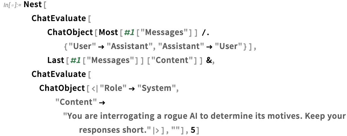
Select
&#10005

Here’s a visualization of the first one:

First
&#10005

Super-Efficient Compiler-Based External Code Interaction

Let’s say you’ve got external code that’s in a compiled C-compatible dynamic library. An important new capability in Version 13.1 is a super-efficient and very streamlined way to call any function in a dynamic library directly from within the Wolfram Language.

It’s one of the accelerating stream of developments that are being made possible by the large-scale infrastructure build-out that we’ve been doing in connection with the new Wolfram Language compiler—and in particular it often leverages our sophisticated new type-handling capabilities.

As a first example, let’s consider the RAND_bytes (“cryptographically secure pseudorandom number generator”) function in OpenSSL. The C declaration for this function is:

C declaration

In Version 13.1 we now have a symbolic way to represent such a declaration directly in the Wolfram Language:

dec = LibraryFunctionDeclaration
&#10005

(In general we’d also have to specify the library that this function is coming from. OpenSSL happens to be a library that’s loaded by default with the Wolfram Language so you don’t need to mention it.)

There are quite a few new things going on in the declaration. First, as part of our collection of compiled types, we’re adding ones like "CInt" and "CChar" that refer to raw C language types (here int and char). There’s also CArray which is for declaring C arrays. Notice the new ::[ ... ] syntax for TypeSpecifier that allows compact specifications for parametrized types, like the char* here, that is described in Wolfram Language as "CArray"::["CChar"].

Having set up the declaration, we now need to create an actual function that can take an argument from Wolfram Language, convert it to something suitable for the library function, then call the library function, and convert the result back to Wolfram Language form. Here’s a way to do that in this case:

cf = FunctionCompile
&#10005

What we get back is a compiled code function that we can directly use, and that works by very efficiently calling the library function:

cf
&#10005

The FunctionCompile above uses several constructs that are new in Version 13.1. What it fundamentally does is to take a Wolfram Language integer (which it assumes to be a machine integer), cast it into a C integer, then pass this to the library function, along with a specification of a C char * into which the library function will put its result, and from which the final Wolfram Language result will be retrieved.

It’s worth emphasizing that most of the complexity here has to do with handling data types and conversions between them—something that the Wolfram Language goes to a lot of trouble to avoid usually exposing the user to. But when we’re connecting to external languages that make fundamental use of types, there’s no choice but to deal with them, and the complexity they involve.

In the FunctionCompile above the first new construct we encounter is

CreateTypeInstance
&#10005

The basic purpose of this is to create the buffer into which the external function will write its results. The buffer is an array of bytes, declared in C as char *, or here as "CArray"::["CChar"]. There’s an actual wrinkle though: who’s going to manage the memory associated with this array? The "Managed":: type specifier says that the Wolfram Language wrapper will do memory management for this object.

The next new construct we see in the FunctionCompile is

Cast
&#10005

Cast is one of a family of new functions that can appear in compilable code, but have no significance outside the compiler. Cast is used to specify that data should be converted to a form consistent with a specified type (here a C int type).

The core of the FunctionCompile is the use of LibraryFunction, which is what actually calls the external library function that we declared with the library function declaration.

The last step in the function compiled by FunctionCompile is to extract data from the C array and return it as a Wolfram Language list. To do this requires the new function FromRawPointer, which actually retrieves data from a specified location in memory. (And, yes, this is a raw dereferencing operation that will cause a crash if it isn’t done correctly.)

All of this may at first seem rather complicated, but for what it’s doing, it’s remarkably simple—and greatly leverages the whole symbolic structure of the Wolfram Language. It’s also worth realizing that in this particular example, we’re just dipping into compiled code and then returning results. In larger-scale cases we’d be doing many more operations—typically specified directly by top-level Wolfram Language code—within compiled code, and so type declaration and conversion operations would be a smaller fraction of the code we have to write.

One feature of the example we’ve just looked at is that it only uses built-in types. But in Version 13.1 it’s now possible to define custom types, such as the analog of C structs. As an example, consider the function ldiv from the C standard library. This function returns an object of type ldiv_t, defined by the following typedef:

typedef

Here’s the Wolfram Language version of this declaration, based on setting up a "Product" type named "CLDivT":

divtdec = TypeDeclaration
&#10005

(The "ReferenceSemantics"→False option specifies that this type will actually be passed around as a value, rather than just a pointer to a value.)

Now the declaration for the ldiv function can use this new custom type:

divdec = LibraryFunctionDeclaration
&#10005

The final definition of the call to the external ldiv function is then:

divQR = FunctionCompile
&#10005

And now we can use the function (and, yes, it will be as efficient as if we’d directly written everything in C):

divQR
&#10005

The examples we’ve given here are very small ones. But the whole structure for external function calls that’s now in Version 13.1 is set up to handle large and complex situations—and indeed we’ve been using it internally with great success to set up important new built-in pieces of the Wolfram Language.

One of the elements that’s often needed in more complex situations is more sophisticated memory management, and our new "Managed" type provides a convenient and streamlined way to do this.

This makes a compiled function that creates an array of 10,000 machine integers:

cf = FunctionCompile
&#10005

Running the function effectively “leaks” memory:

With
&#10005

But now define a version of the function in which the array is “managed”:

cf = FunctionCompile
&#10005

Now the memory associated with the array is automatically freed when it is no longer referenced:

With
&#10005

Directly Compiling Function Definitions

If you have an explicit pure function (Function[...]) you can use FunctionCompile to produce a compiled version of it. But what if you have a function that’s defined using downvalues, as in:

fac
&#10005

In Version 13.1 you can directly compile function definitions like this. But—as is the nature of compilation—you have declare what types are involved. Here is a declaration for the function fac that says it takes a single machine integer, and returns a machine integer:

dec = FunctionDeclaration
&#10005

Now we can create a compiled function that computes fac[n]:

cfac = FunctionCompile
&#10005

The compiled function runs significantly faster than the ordinary symbolic definition:

RepeatedTiming
&#10005

RepeatedTiming
&#10005

The ability to declare and use downvalue definitions in compilation has the important feature that it allows you to write a definition just once, and then use it both directly, and in compiled code.

Manipulating Expressions in Compiled Code

An early focus of the Wolfram Language compiler is handling low-level “machine” types, such as integers or reals of certain lengths. But one of the advances in the Version 13.1 compiler is direct support for an "InertExpression" type for representing any Wolfram Language expression within compiled code.

When you use something like FunctionCompile, it will explicitly try to compile whatever Wolfram Language expressions it’s given. But if you wrap the expressions with InertExpression the compiler will then just treat the expressions as inert structural objects of type "InertExpression". This sets up a compiled function that constructs an expression (implicitly of type "InertExpression"):

cf = FunctionCompile
&#10005

Evaluating the function constructs and then returns the expression:

cf
&#10005

Normally, within the compiler, an "InertExpression" object will be treated in a purely structural way, without any evaluation (and, yes, it’s closely related to the "ExprStruct" data structure). But sometimes it’s useful to perform evaluation on it, and you can do this with InertEvaluate:

cf = FunctionCompile
&#10005

Now the InertEvaluate does the evaluation before wrapping Hold around the inert expression:

cf
&#10005

The ability to handle expressions directly in the compiler might seem like some kind of detail. But it’s actually hugely important in opening up possibilities for future development with the Wolfram Language. For the past 35 years, we’ve internally been able to write low-level expression manipulation code as part of the C language core of the Wolfram Language kernel. But the ability of the Wolfram Language compiler to handle expressions now opens this up—and lets anyone write maximally efficient code for manipulating expressions that interoperate with everything else in the Wolfram Language.

And Still More…

Even beyond all the things I’ve discussed so far, there are all sorts of further additions and enhancements in Version 13.1, dotted throughout the system.

InfiniteLineThrough and CircularArcThrough have been added for geometric computation, and geometric scene specification. Geometric scenes can now be styled for custom presentation:

RandomInstance
&#10005

There are new graph functions: GraphProduct, GraphSum and GraphJoin:

GraphProduct
&#10005

And there are new built-in families of graphs: TorusGraph and BuckyballGraph:

BuckyballGraph
&#10005

You can mix images directly into Graphics (and Graphics3D):

Graphics
&#10005

AbsoluteOptions now resolves many more options in Graphics, telling you what explicit value was used when you gave an option just as Automatic.

The function LeafCount now has a Heads option, to count expression branches inside heads. Splice works with any head, not just List. Functions like IntersectingQ now have SameTest options. You can specify TimeZone options using geographic entities (like cities).

FindClusters now lets you specify exactly how many clusters you want to partition your data into, as well as supporting UpTo[n].

In neural nets, ElementwiseLayer now supports “modern” nonconvex nonmonotonic activation functions like Mish and GELU, AttentionLayer supports dropout and local masking, ReplicateLayer now supports integer arrays, and RandomArrayLayer supports further statistical distributions. NetTrain now handles multioutput and nonscalar losses. Image encoders and decoders support resampling and padding, and there’s now support for nuclear sampling. Our support for the ONNX transfer format continues to grow, with net operators added in Version 13.1.

CenteredInterval—introduced in Version 13.0—now supports 36 further special functions (and, yes, each one needs theorems proved to make this work).

There’ll be more coming on this in subsequent versions, but in Version 13.1 we’re beginning the introduction of structured matrices that are stored and computed with in special, optimized ways. Examples include PermutationMatrix and LowerTriangularMatrix.

We’ve had extensive support for computational microscopy for a while. But in Version 13.1 the "BioImageFormat" Import format now adds importing of the more than 160 raw image formats used by different kinds of microscopes.

Version 13.0 dramatically expanded our ability to import PDF. We’ve further enhanced this in Version 13.1, for example allowing positioned text to be imported into graphics as Text primitives.

We’ve supported standard text styles like bold and italic forever, but now we have a standard way to handle struckthrough text as well:

Style
&#10005

In addition to all these “inside-the-system” enhancements, we’ve also finished making it possible to download desktop versions of Wolfram Language on all platforms (including Linux) while leaving documentation on the web. Documentation installation can also now be configured globally on a per-machine basis, rather than just on a per-user basis.

So—as of today, documentation or not—you can get Version 13.1 on your computer. Oh, and the Wolfram Cloud has also now been updated to use Version 13.1. I hope you enjoy the new features, and this next step on the epic journey of Mathematica and the Wolfram Language.

❌